This is an example of interfacing R and shiny to allow users to explore a biological model often encountered in an introductory ecology class. We are interested the growth of a population that is composed of multiple, discrete stages or age classes. Patrick H. Leslie provides an in-depth derivation of the model in a 1945 paper (Leslie 1945).
The population at time \(t\) is represented by a vector \(\bar{x}_t\), where each element of the vector represents the number of individuals in each age class (e.g. if a population has \(n\) age classes, then \(\bar{x}_t\) has \(n\) elements). Time is considered discrete and we assume that the population is censused prior to breeding. We assume that individuals within each age class are identical, and that each has some probability of maturing to the next age class, surviving (staying in the same age class), and reproduction. Changes in the population from one timestep to another are represented as:
\[\bar{x}_{t+1}=L\bar{x}_t\]
where \(L\) is an \(n\) x \(n\) Leslie matrix (or more generally, a projection matrix) that describes the contribution of each age class to the population at time \(t+1\).
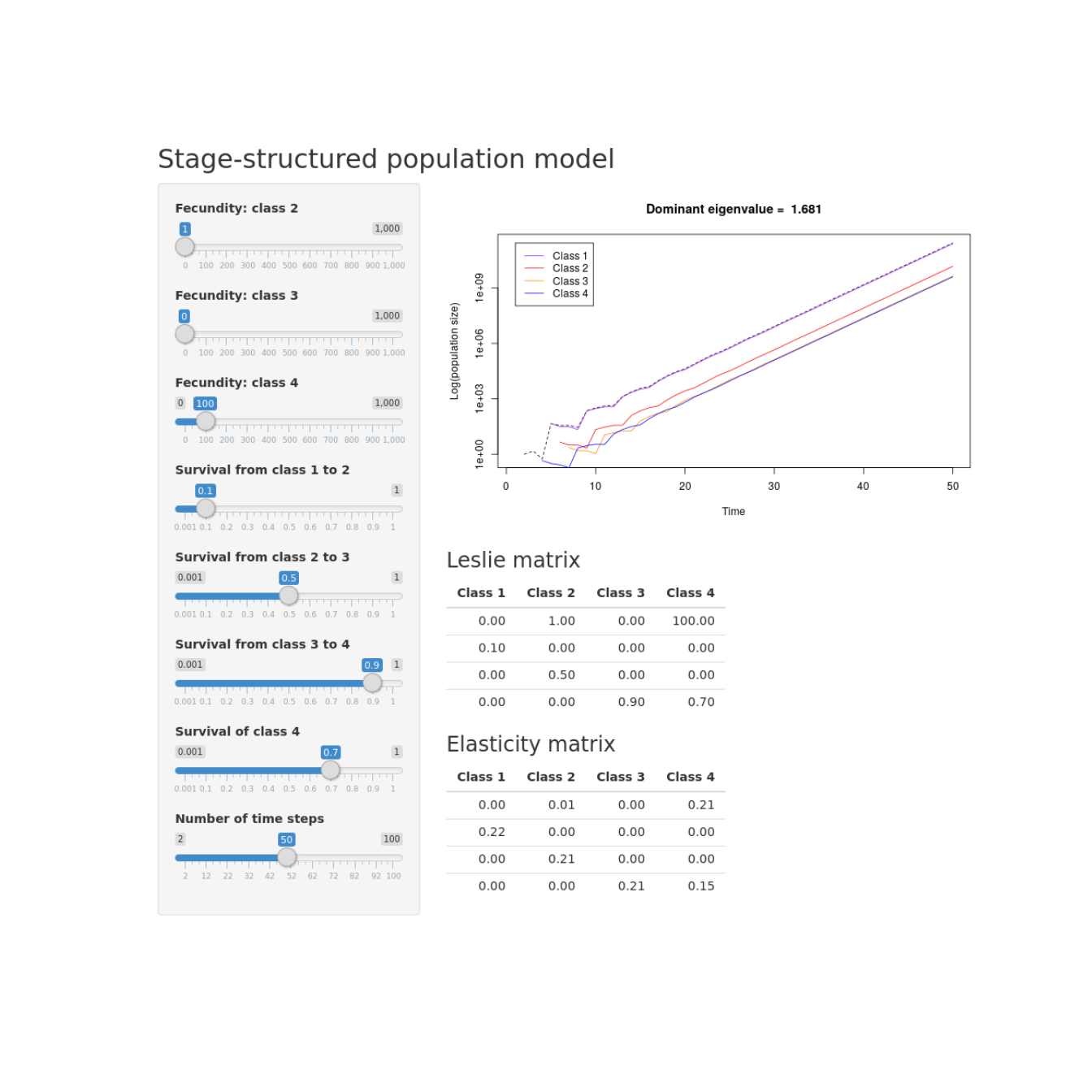
Suppose we are tasked with modeling the annual dynamics of a population with four age classes, and \(t\) represents years. For simplicity, we model only females and assume that plenty of males are available for breeding. Individuals in the first age class survive to class 2 with probability 0.1, class 2 individuals survive to class 3 with probability 0.5, class 3 individuals survive to class 4 with probability 0.9, and class four individuals survive each year with probability 0.7. Only the fourth age class is reproductive, with individuals producing 100 class 1 individuals per year.
Equivalently, as a Leslie matrix:
\[\left[\begin{array}{rrrr} 0 & 0 & 0 & 100 \\ .1 & 0 & 0 & 0 \\ 0 & .5 & 0 & 0 \\ 0 & 0 & .9 & .7 \end{array}\right]\]
The long term population growth rate is related to the dominant eigenvalue \(\lambda_{1}\) of \(L\). If \[\lambda_{1} < 1\], the population declines to extinction, and if \[\lambda_{1} > 1\] the population increases.
From a management perspective, it is often useful to know how limited resources may be allocated to increase population growth or prevent extinction. In other words, if an element \[l_{ij}\] such as fecundity or survival could be manipulated by managers, how much would the long term population growth rate change? To this end, one can calculate the sensitivity of the dominant eigenvalue to small changes in \(l_{ij}\):
\[ \frac{\partial \lambda_{1}}{\partial l_{ij}} = \frac{(w_{1}){i}(v_{1})_{j}}{\bar{w}_{1}^{T} \bar{v}_{1}} \]
where \(w_1\) and \(v_1\) are left and right eigenvectors, respectively, associated with the dominant eigenvalue. Because survival and fecundity are on different scales, sensitivity is often scaled by a factor of \(\frac{L_{ij}}{\lambda_1}\) for a measure of elasticity.
The shiny app
Files are accessible in this repository. Please feel free to clone for your own use and/or contribute.
Here is a link to the resulting app.