This post is intended to provide a simple example of how to construct and make inferences on a multi-species multi-year occupancy model using R, JAGS, and the ‘rjags’ package. This is not intended to be a standalone tutorial on dynamic community occupancy modeling (MacKenzie et al. 2002; Royle and Kéry 2007; Kéry and Royle 2008; Dorazio et al. 2010). Royle and Dorazio’s Hierarchichal Modeling and Inference in Ecology also provides a clear explanation of simple one species occupancy models, multispecies occupancy models, and dynamic (multiyear) occupancy models, among other things (Royle and Dorazio 2008). There’s also a wealth of code provided here by Elise Zipkin, J. Andrew Royle, and others.
Before getting started, we can define two convenience functions:
Then, initializing the number of sites, species, years, and repeat surveys (i.e. surveys within years, where the occupancy status of a site is assumed to be constant),
nsite <- 20
nspec <- 3
nyear <- 4
nrep <- 2
we can begin to consider occupancy. We’re interested in making inferences about the rates of colonization and population persistence for each species in a community, while estimating and accounting for imperfect detection.
Occupancy status at site \(j\), by species \(i\), in year \(t\) is represented by \(z(j,i,t)\). For occupied sites \(z=1\); for unoccupied sites \(z=0\). However, \(Z\) is incompletely observed: it is possible that a species \(i\) is present at a site \(j\) in some year \(t\) (\(z(j,i,t)=1\)) but species \(i\) was never seen at at site \(j\) in year \(t\) across all \(k\) repeat surveys because of imperfect detection. These observations are represented by \(x(j,i,t,k)\). Here we assume that there are no “false positive” observations. In other words, if \(\sum_{1}^{k}x(j,i,t,k)>0\) , then \(z(j,i,t)=1\). If a site is occupied, the probability that \(x(j,i,t,k)=1\) is represented as a Bernoulli trial with probability of detection \(p(j,i,t,k)\), such that
\[ x(j,i,t,k) \sim \text{Bernoulli}(z(j,i,t)p(j,i,t,k)) \]
The occupancy status \(z\) of species \(i\) at site \(j\) in year \(t\) is modeled as a Markov Bernoulli trial. In other words whether a species is present at a site in year \(t\) is influenced by whether it was present at year \(t−1\).
\[ z(j,i,t) \sim \text{Bernoulli}(\psi(j,i,t)) \]
where for \(t>1\)
\[ \text{logit}(\psi_{j,i,t})=\beta_i + \rho_i z(i, j, t-1) \]
and in year one \((t=1)\)
\[ \text{logit}(\psi_{j,i,1})=\beta_i + \rho_i z_0(i, j) \]
where the occupancy status in year 0, \(z_0(i,j) \sim \text{Bernoulli}(\rho_{0i})\), and \(\rho_{0i} \sim \text{Uniform}(0,1)\). \(\beta_i\) and \(\rho_i\) are parameters that control the probabilities of colonization and persistence. If a site was unoccupied by species \(i\) in a previous year \(z(i,j,t−1)=0\), then the probability of colonization is given by the antilogit of \(\beta_i\). If a site was previously occupied \(z(i,j,t−1)=1\), the probability of population persistence is given by the anitlogit of \(\beta_i + \rho_i\). We assume that the distributions of species specific parameters are defined by community level hyperparameters such that \(\beta_i \sim \text{Normal}(\mu_\beta, \sigma_\beta)\) and \(rho_i \sim \text{Normal}(\mu_\rho, \sigma_\rho)\). We can generate occupancy data as follows:
# community level hyperparameters
mubeta <- 1
sdbeta <- 0.2

murho <- -2
sdrho <- .1

# species specific random effects
set.seed(1)  # for reproducibility
beta <- rnorm(nspec, mubeta, sdbeta)
set.seed(1008)
rho <- rnorm(nspec, murho, sdrho)

# initial occupancy states
set.seed(237)
rho0 <- runif(nspec, 0, 1)
z0 <- array(dim = c(nsite, nspec))
for (i in 1:nspec) {
    z0[, i] <- rbinom(nsite, 1, rho0[i])
}

# subsequent occupancy
z <- array(dim = c(nsite, nspec, nyear))
lpsi <- array(dim = c(nsite, nspec, nyear))
psi <- array(dim = c(nsite, nspec, nyear))
for (j in 1:nsite) {
    for (i in 1:nspec) {
        for (t in 1:nyear) {
            if (t == 1) {
                lpsi[j, i, t] <- beta[i] + rho[i] * z0[j, i]
                psi[j, i, t] <- antilogit(lpsi[j, i, t])
                z[j, i, t] <- rbinom(1, 1, psi[j, i, t])
            } else {
                lpsi[j, i, t] <- beta[i] + rho[i] * z[j, i, t - 1]
                psi[j, i, t] <- antilogit(lpsi[j, i, t])
                z[j, i, t] <- rbinom(1, 1, psi[j, i, t])
            }
        }
    }
}
For simplicity, we’ll assume that there are no differences in species detectability among sites, years, or repeat surveys, but that detectability varies among species. We’ll again use hyperparameters to specify a distribution of detection probabilities in our community, such that \(\text{logit}(p_i) \sim \text{Normal}(\mu_p, \sigma_p)\).
We can now generate our observations based on occupancy states and detection probabilities. Although this could be vectorized for speed, let’s stick with nested for loops in the interest of clarity.
Now that we’ve collected some data, we can specify our model:
cat("
model{
  #### priors
  # beta hyperparameters
  p_beta ~ dbeta(1, 1)
  mubeta <- log(p_beta / (1 - p_beta))
  sigmabeta ~ dunif(0, 10)
  taubeta <- (1 / (sigmabeta * sigmabeta))

  # rho hyperparameters
  p_rho ~ dbeta(1, 1)
  murho <- log(p_rho / (1 - p_rho))
  sigmarho~dunif(0,10)
  taurho<-1/(sigmarho*sigmarho)

  # p hyperparameters
  p_p ~ dbeta(1, 1)
  mup <- log(p_p / (1 - p_p))
  sigmap ~ dunif(0,10)
  taup <- (1 / (sigmap * sigmap))

  #### occupancy model
  # species specific random effects
  for (i in 1:(nspec)) {
    rho0[i] ~ dbeta(1, 1)
    beta[i] ~ dnorm(mubeta, taubeta)
    rho[i] ~ dnorm(murho, taurho)
  }

  # occupancy states
  for (j in 1:nsite) {
    for (i in 1:nspec) {
      z0[j, i] ~ dbern(rho0[i])
      logit(psi[j, i, 1]) <- beta[i] + rho[i] * z0[j, i]
      z[j, i, 1] ~ dbern(psi[j, i, 1])
      for (t in 2:nyear) {
        logit(psi[j, i, t]) <- beta[i] + rho[i] * z[j, i, t-1]
        z[j, i, t] ~ dbern(psi[j, i, t])
      }
    }
  }

  #### detection model
  for(i in 1:nspec){
    lp[i] ~ dnorm(mup, taup)
    p[i] <- (exp(lp[i])) / (1 + exp(lp[i]))
  }

  #### observation model
  for (j in 1:nsite){
    for (i in 1:nspec){
      for (t in 1:nyear){
        mu[j, i, t] <- z[j, i, t] * p[i]
        for (k in 1:nrep){
          x[j, i, t, k] ~ dbern(mu[j, i, t])
        }
      }
    }
  }
}
", fill=TRUE, file="com_occ.txt")
Next, bundle up the data.
data <- list(x = x, nrep = nrep, nsite = nsite, nspec = nspec, nyear = nyear)Provide initial values.
zinit <- array(dim = c(nsite, nspec, nyear))
for (j in 1:nsite) {
    for (i in 1:nspec) {
        for (t in 1:nyear) {
            zinit[j, i, t] <- max(x[j, i, t, ])
        }
    }
}

inits <- function() {
    list(p_beta = runif(1, 0, 1), p_rho = runif(1, 0, 1), sigmarho = runif(1,
        0, 1), sigmap = runif(1, 0, 10), sigmabeta = runif(1, 0, 10), z = zinit)
}
As a side note, it is helpful in JAGS to provide initial values for the
incompletely observed occupancy state \(z\) that are consistent with observed
presences, as provided in this example with zinit. In other words if
\(x(j,i,t,k)=1\), provide an intial value of 1 for \(z(j,i,t)\). Unlike WinBUGS and
OpenBUGS, if you do not do this, you’ll often (but not always) encounter an
error message such as:
# Error in jags.model(file = 'com_occ.txt', data = data, n.chains = 3) :
# Error in node x[1,1,2,3] Observed node inconsistent with unobserved
# parents at initialization
Now we’re ready to monitor and make inferences about some parameters of interest using JAGS.
params <- c("lp", "beta", "rho")
ocmod <- jags.model(file = "com_occ.txt", inits = inits, data = data,
                    n.chains = 2)
Compiling model graph
Resolving undeclared variables
Allocating nodes
Graph information:
Observed stochastic nodes: 480
Unobserved stochastic nodes: 318
Total graph size: 1789
Initializing model
|
| | 0%
|
|+ | 2%
|
|++ | 4%
|
|+++ | 6%
|
|++++ | 8%
|
|+++++ | 10%
|
|++++++ | 12%
|
|+++++++ | 14%
|
|++++++++ | 16%
|
|+++++++++ | 18%
|
|++++++++++ | 20%
|
|+++++++++++ | 22%
|
|++++++++++++ | 24%
|
|+++++++++++++ | 26%
|
|++++++++++++++ | 28%
|
|+++++++++++++++ | 30%
|
|++++++++++++++++ | 32%
|
|+++++++++++++++++ | 34%
|
|++++++++++++++++++ | 36%
|
|+++++++++++++++++++ | 38%
|
|++++++++++++++++++++ | 40%
|
|+++++++++++++++++++++ | 42%
|
|++++++++++++++++++++++ | 44%
|
|+++++++++++++++++++++++ | 46%
|
|++++++++++++++++++++++++ | 48%
|
|+++++++++++++++++++++++++ | 50%
|
|++++++++++++++++++++++++++ | 52%
|
|+++++++++++++++++++++++++++ | 54%
|
|++++++++++++++++++++++++++++ | 56%
|
|+++++++++++++++++++++++++++++ | 58%
|
|++++++++++++++++++++++++++++++ | 60%
|
|+++++++++++++++++++++++++++++++ | 62%
|
|++++++++++++++++++++++++++++++++ | 64%
|
|+++++++++++++++++++++++++++++++++ | 66%
|
|++++++++++++++++++++++++++++++++++ | 68%
|
|+++++++++++++++++++++++++++++++++++ | 70%
|
|++++++++++++++++++++++++++++++++++++ | 72%
|
|+++++++++++++++++++++++++++++++++++++ | 74%
|
|++++++++++++++++++++++++++++++++++++++ | 76%
|
|+++++++++++++++++++++++++++++++++++++++ | 78%
|
|++++++++++++++++++++++++++++++++++++++++ | 80%
|
|+++++++++++++++++++++++++++++++++++++++++ | 82%
|
|++++++++++++++++++++++++++++++++++++++++++ | 84%
|
|+++++++++++++++++++++++++++++++++++++++++++ | 86%
|
|++++++++++++++++++++++++++++++++++++++++++++ | 88%
|
|+++++++++++++++++++++++++++++++++++++++++++++ | 90%
|
|++++++++++++++++++++++++++++++++++++++++++++++ | 92%
|
|+++++++++++++++++++++++++++++++++++++++++++++++ | 94%
|
|++++++++++++++++++++++++++++++++++++++++++++++++ | 96%
|
|+++++++++++++++++++++++++++++++++++++++++++++++++ | 98%
|
|++++++++++++++++++++++++++++++++++++++++++++++++++| 100%nburn <- 10000
update(ocmod, n.iter = nburn)
  |
  |                                                  |   0%
  |
  |*                                                 |   2%
  |
  |**                                                |   4%
  |
  |***                                               |   6%
  |
  |****                                              |   8%
  |
  |*****                                             |  10%
  |
  |******                                            |  12%
  |
  |*******                                           |  14%
  |
  |********                                          |  16%
  |
  |*********                                         |  18%
  |
  |**********                                        |  20%
  |
  |***********                                       |  22%
  |
  |************                                      |  24%
  |
  |*************                                     |  26%
  |
  |**************                                    |  28%
  |
  |***************                                   |  30%
  |
  |****************                                  |  32%
  |
  |*****************                                 |  34%
  |
  |******************                                |  36%
  |
  |*******************                               |  38%
  |
  |********************                              |  40%
  |
  |*********************                             |  42%
  |
  |**********************                            |  44%
  |
  |***********************                           |  46%
  |
  |************************                          |  48%
  |
  |*************************                         |  50%
  |
  |**************************                        |  52%
  |
  |***************************                       |  54%
  |
  |****************************                      |  56%
  |
  |*****************************                     |  58%
  |
  |******************************                    |  60%
  |
  |*******************************                   |  62%
  |
  |********************************                  |  64%
  |
  |*********************************                 |  66%
  |
  |**********************************                |  68%
  |
  |***********************************               |  70%
  |
  |************************************              |  72%
  |
  |*************************************             |  74%
  |
  |**************************************            |  76%
  |
  |***************************************           |  78%
  |
  |****************************************          |  80%
  |
  |*****************************************         |  82%
  |
  |******************************************        |  84%
  |
  |*******************************************       |  86%
  |
  |********************************************      |  88%
  |
  |*********************************************     |  90%
  |
  |**********************************************    |  92%
  |
  |***********************************************   |  94%
  |
  |************************************************  |  96%
  |
  |************************************************* |  98%
  |
  |**************************************************| 100%
out <- coda.samples(ocmod, n.iter = 10000, variable.names = params)
|
| | 0%
|
|* | 2%
|
|** | 4%
|
|*** | 6%
|
|**** | 8%
|
|***** | 10%
|
|****** | 12%
|
|******* | 14%
|
|******** | 16%
|
|********* | 18%
|
|********** | 20%
|
|*********** | 22%
|
|************ | 24%
|
|************* | 26%
|
|************** | 28%
|
|*************** | 30%
|
|**************** | 32%
|
|***************** | 34%
|
|****************** | 36%
|
|******************* | 38%
|
|******************** | 40%
|
|********************* | 42%
|
|********************** | 44%
|
|*********************** | 46%
|
|************************ | 48%
|
|************************* | 50%
|
|************************** | 52%
|
|*************************** | 54%
|
|**************************** | 56%
|
|***************************** | 58%
|
|****************************** | 60%
|
|******************************* | 62%
|
|******************************** | 64%
|
|********************************* | 66%
|
|********************************** | 68%
|
|*********************************** | 70%
|
|************************************ | 72%
|
|************************************* | 74%
|
|************************************** | 76%
|
|*************************************** | 78%
|
|**************************************** | 80%
|
|***************************************** | 82%
|
|****************************************** | 84%
|
|******************************************* | 86%
|
|******************************************** | 88%
|
|********************************************* | 90%
|
|********************************************** | 92%
|
|*********************************************** | 94%
|
|************************************************ | 96%
|
|************************************************* | 98%
|
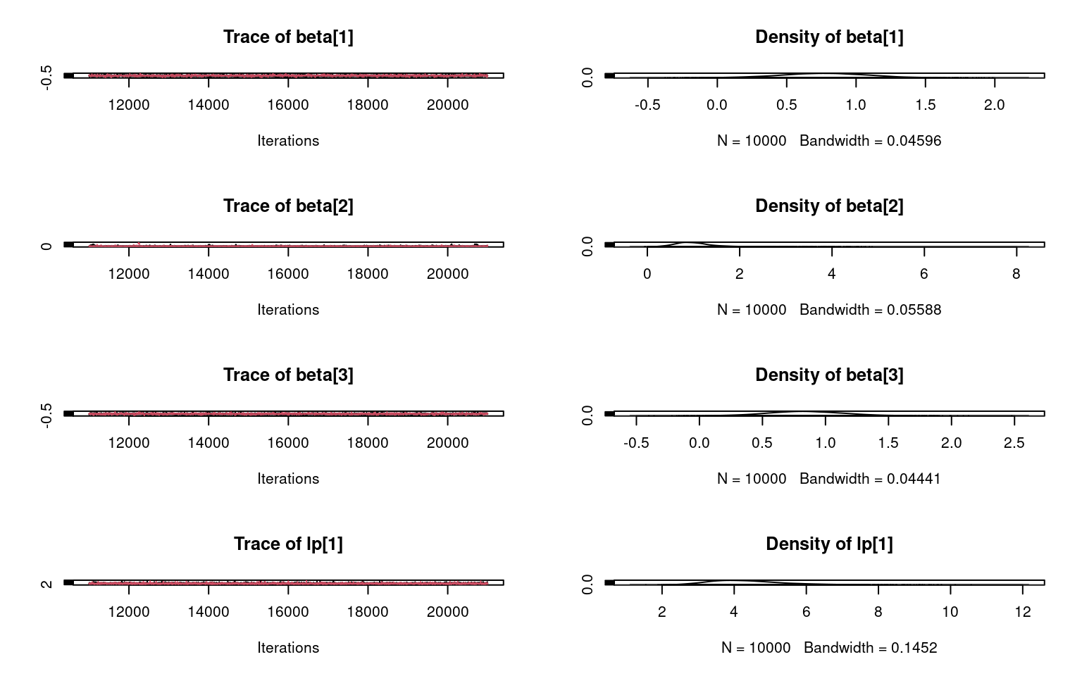
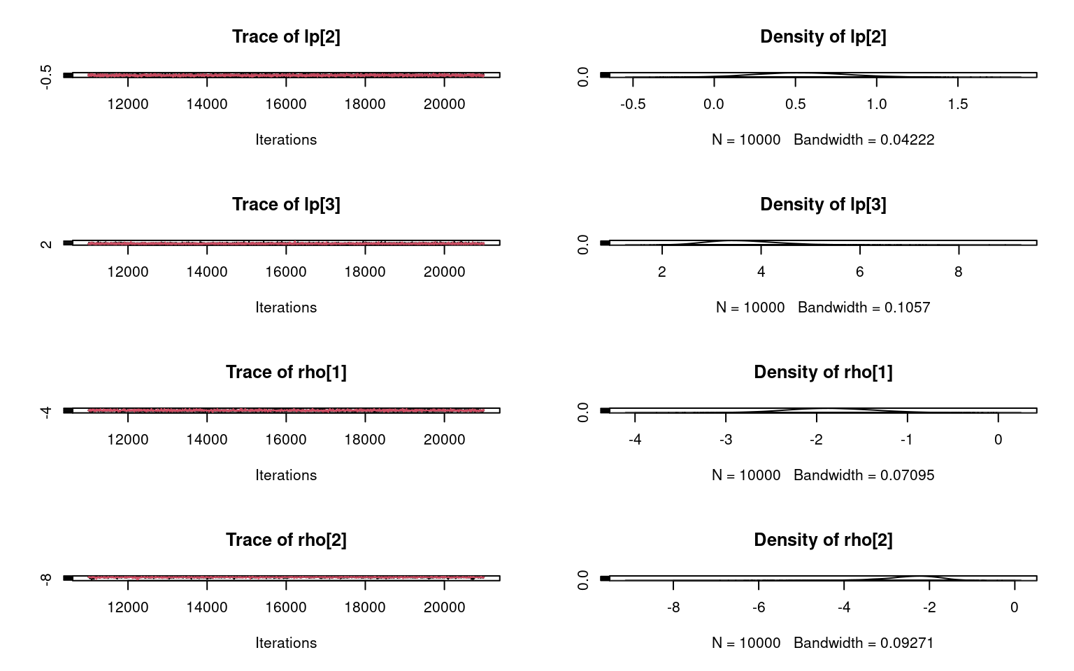
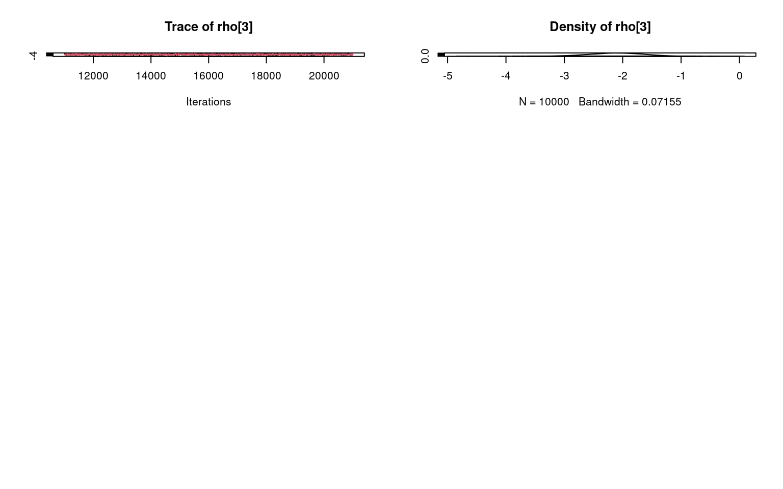
|**************************************************| 100%summary(out)
Iterations = 11001:21000
Thinning interval = 1
Number of chains = 2
Sample size per chain = 10000

1. Empirical mean and standard deviation for each variable,
   plus standard error of the mean:

           Mean     SD Naive SE Time-series SE
beta[1]  0.7679 0.3173 0.002244       0.007803
beta[2]  1.0692 0.5820 0.004115       0.025065
beta[3]  0.8474 0.3079 0.002177       0.006865
lp[1]    4.3725 1.0684 0.007555       0.012143
lp[2]    0.5402 0.2887 0.002041       0.004442
lp[3]    3.6732 0.7496 0.005301       0.007816
rho[1]  -1.8426 0.4896 0.003462       0.011560
rho[2]  -2.4753 0.7493 0.005298       0.025575
rho[3]  -2.1264 0.4960 0.003507       0.010948

2. Quantiles for each variable:

            2.5%     25%     50%     75%   97.5%
beta[1]  0.13043  0.5613  0.7683  0.9823  1.3799
beta[2]  0.32801  0.7354  0.9671  1.2474  2.5356
beta[3]  0.25697  0.6404  0.8386  1.0473  1.4730
lp[1]    2.72967  3.6221  4.2195  4.9523  6.8553
lp[2]   -0.01461  0.3429  0.5351  0.7323  1.1189
lp[3]    2.41727  3.1468  3.5942  4.1151  5.3536
rho[1]  -2.78718 -2.1701 -1.8526 -1.5200 -0.8629
rho[2]  -4.23507 -2.8309 -2.3688 -1.9814 -1.3360
rho[3] -3.14440 -2.4444 -2.1116 -1.7889 -1.2037plot(out)