People love \(R^2\). As such, when Nakagawa and Schielzeth published
A general and simple method for obtaining \(R^2\) from generalized linear
mixed-effects models in Methods in Ecology and Evolution earlier this year
(Nakagawa and Schielzeth 2013),
ecologists (amid increasing use of generalized linear mixed models (GLMMs))
rejoiced. Now there’s
an R function that automates \(R^2\) calculations for GLMMs fit with the lme4 package.
\(R^2\) is usually reported as a point estimate of the variance explained by a model, using the maximum likelihood estimates of the model parameters and ignoring uncertainty around these estimates. Nakagawa and Schielzeth (2013) noted that it may be desirable to quantify the uncertainty around \(R^2\) using MCMC sampling. So, here we are.
Background
\(R^2\) quantifies the proportion of observed variance explained by a statistical model. When it is large (near 1), much of the variance in the data is explained by the model.
Nakagawa and Schielzeth (2013) present two \(R^2\) statistics for generalized linear mixed models:
- Marginal \(R^2_{GLMM(m)}\), which represents the proportion of variance explained by fixed effects:
\[R^2_{GLMM(m)} = \frac{\sigma^2_f}{\sigma^2_f + \sum_{l=1}^{u}\sigma^2_l + \sigma^2_d + \sigma^2_e}\]
where \(\sigma^2_f\) represents the variance in the fitted values (on a link scale) based on the fixed effects:
\[ \sigma^2_f = var(\boldsymbol{X \beta}) \]
\(\boldsymbol{X}\) is the design matrix of the fixed effects, and \(\boldsymbol{\beta}\) is the vector of fixed effects estimates.
\(\sum_{l=1}^{u}\sigma^2_l\) represents the sum the variance components for all of \(u\) random effects. \(\sigma^2_d\) is the distribution-specific variance (Nakagawa and Schielzeth 2010), and \(\sigma^2_e\) represents added dispersion.
- Conditional \(R^2_{GLMM(c)}\) represents the proportion of variance explained by the fixed and random effects combined:
\[ R^2_{GLMM(c)} = \frac{\sigma^2_f + \sum_{l=1}^{u}\sigma^2_l}{\sigma^2_f + \sum_{l=1}^{u}\sigma^2_l + \sigma^2_d + \sigma^2_e} \]
Point-estimation of \(R^2_{GLMM}\)
Here, I’ll follow the example of an overdispersed Poisson GLMM provided in the supplement to Nakagawa & Schielzeth (Nakagawa and Schielzeth 2013). This is their most complicated example, and the simpler ones ought to be relatively straightforward for those that are interested in normal or binomial GLMMs.
library(arm)
library(ggmcmc)
library(lme4)
library(rjags)

# First, simulate data (code adapted from Nakagawa & Schielzeth 2013):
n_population <- 8
n <- 100
Population <- gl(n_population, k = n / n_population, n)

n_container <- 10
Container <- gl(n_container, n / n_container, n)

# Sex of the individuals. Uni-sex within each container (individuals are
# sorted at the pupa stage)
Sex <- factor(sample(c("Female", "Male"), n, replace = TRUE))

# Habitat at the collection site: dry or wet soil (four indiviudal from
# each Habitat in each container)
Habitat <- factor(sample(c("dry", "wet"), n, replace = TRUE))

# Food treatment at the larval stage: special food ('Exp') or standard
# food ('Cont')
Treatment <- factor(sample(c("Cont", "Exp"), n, replace = TRUE))

# Data combined in a dataframe
Data <- data.frame(Population = Population,
    Container = Container, Sex = Sex,
    Habitat = Habitat, Treatment = Treatment)

# Subset the design matrix (only females express colour morphs)
DataF <- Data[Data$Sex == "Female", ]

# random effects
PopulationE <- rnorm(n_population, 0, sqrt(0.4))
ContainerE <- rnorm(n_container, 0, sqrt(0.05))

# generation of response values on link scale (!) based on fixed effects,
# random effects and residual errors
EggLink <- with(DataF,
                  1.1 +
                  0.5 * (as.numeric(Treatment) - 1) +
                  0.1 * (as.numeric(Habitat) - 1) +
                  PopulationE[Population] +
                  ContainerE[Container])

# data generation (on data scale!) based on Poisson distribution
DataF$Egg <- rpois(length(EggLink), exp(EggLink))
Having simulated a dataset, calculate the \(R^2\) point-estimates, using the lme4 package to fit the model.
# Creating a dummy variable that allows estimating additive dispersion in
# glmer This triggers a warning message when fitting the model
Unit <- factor(1:length(DataF$Egg))

# Fit null model without fixed effects (but including all random effects)
m0 <- glmer(Egg ~ 1 + (1 | Population) + (1 | Container) + (1 | Unit),
    family = "poisson", data = DataF)

# Fit alternative model including fixed and all random effects
mF <- glmer(Egg ~ Treatment + Habitat + (1 | Population) + (1 | Container) +
    (1 | Unit), family = "poisson", data = DataF)

# View model fits for both models
summary(m0)
Generalized linear mixed model fit by maximum likelihood (Laplace
Approximation) [glmerMod]
Family: poisson ( log )
Formula: Egg ~ 1 + (1 | Population) + (1 | Container) + (1 | Unit)
Data: DataF
AIC BIC logLik deviance df.resid
257.7 265.8 -124.9 249.7 51
Scaled residuals:
Min 1Q Median 3Q Max
-1.5910 -0.5656 -0.3137 0.5858 1.7928
Random effects:
Groups Name Variance Std.Dev.
Unit (Intercept) 4.377e-08 0.0002092
Container (Intercept) 5.213e-07 0.0007220
Population (Intercept) 4.986e-01 0.7061462
Number of obs: 55, groups: Unit, 55; Container, 10; Population, 8
Fixed effects:
Estimate Std. Error z value Pr(>|z|)
(Intercept) 1.5526 0.2604 5.962 2.49e-09 ***
---
Signif. codes: 0 '***' 0.001 '**' 0.01 '*' 0.05 '.' 0.1 ' ' 1
optimizer (Nelder_Mead) convergence code: 0 (OK)
Model failed to converge with max|grad| = 0.00622563 (tol = 0.002, component 1)summary(mF)Generalized linear mixed model fit by maximum likelihood (Laplace
Approximation) [glmerMod]
Family: poisson ( log )
Formula:
Egg ~ Treatment + Habitat + (1 | Population) + (1 | Container) +
(1 | Unit)
Data: DataF
AIC BIC logLik deviance df.resid
257.9 269.9 -122.9 245.9 49
Scaled residuals:
Min 1Q Median 3Q Max
-1.51389 -0.55034 -0.08826 0.47550 2.07213
Random effects:
Groups Name Variance Std.Dev.
Unit (Intercept) 0.0000 0.0000
Container (Intercept) 0.0000 0.0000
Population (Intercept) 0.4939 0.7028
Number of obs: 55, groups: Unit, 55; Container, 10; Population, 8
Fixed effects:
Estimate Std. Error z value Pr(>|z|)
(Intercept) 1.42059 0.27659 5.136 2.81e-07 ***
TreatmentExp 0.23000 0.11652 1.974 0.0484 *
Habitatwet 0.05464 0.11964 0.457 0.6479
---
Signif. codes: 0 '***' 0.001 '**' 0.01 '*' 0.05 '.' 0.1 ' ' 1
Correlation of Fixed Effects:
(Intr) TrtmnE
TreatmntExp -0.232
Habitatwet -0.292 0.153
optimizer (Nelder_Mead) convergence code: 0 (OK)
boundary (singular) fit: see help('isSingular')# Extraction of fitted value for the alternative model fixef() extracts
# coefficents for fixed effects model.matrix(mF) returns design matrix
Fixed <- fixef(mF)[2] * model.matrix(mF)[, 2] + fixef(mF)[3] * model.matrix(mF)[, 3]
# Calculation of the variance in fitted values
VarF <- var(Fixed)
# An alternative way for getting the same result
VarF <- var(as.vector(fixef(mF) %*% t(model.matrix(mF))))
# R2GLMM(m) - marginal R2GLMM see Equ. 29 and 30 and Table 2 fixef(m0)
# returns the estimate for the intercept of null model
R2m <- VarF/(VarF + VarCorr(mF)$Container[1] +
VarCorr(mF)$Population[1] + VarCorr(mF)$Unit[1] +
log(1 + 1/exp(as.numeric(fixef(m0))))
)
# R2GLMM(c) - conditional R2GLMM for full model Equ. XXX, XXX
R2c <- (VarF + VarCorr(mF)$Container[1] + VarCorr(mF)$Population[1])/
(VarF + VarCorr(mF)$Container[1] + VarCorr(mF)$Population[1] +
VarCorr(mF)$Unit[1] + log(1 + 1/exp(as.numeric(fixef(m0))))
)
# Print marginal and conditional R-squared values
cbind(R2m, R2c) R2m R2c
[1,] 0.0181809 0.7251428Having stored our point estimates, we can now turn to Bayesian methods instead, and generate \(R^2\) posteriors.
Posterior uncertainty in \(R^2_{GLMM}\)
We need to fit two models in order to get the needed parameters for \(R^2_{GLMM}\). First, a model that includes all random effects, but only an intercept fixed effect is fit to estimate the distribution specific variance \(\sigma^2_d\). Second, we fit a model that includes all random and all fixed effects to estimate the remaining variance components.
First I’ll clean up the data that we’ll feed to JAGS:
# Prepare the data
jags_d <- as.list(DataF)[-c(2, 3)]  # redefine container, don't need sex
jags_d$nobs <- nrow(DataF)
jags_d$npop <- length(unique(jags_d$Population))

# renumber containers from 1:ncontainer for ease of indexing
jags_d$Container <- rep(NA, nrow(DataF))
for (i in 1:nrow(DataF)) {
  jags_d$Container[i] <- which(unique(DataF$Container) == DataF$Container[i])
}
jags_d$ncont <- length(unique(jags_d$Container))

# Convert binary factors to 0's and 1's
jags_d$Habitat <- ifelse(jags_d$Habitat == "dry", 0, 1)
jags_d$Treatment <- ifelse(jags_d$Treatment == "Cont", 0, 1)
str(jags_d)
List of 8
$ Population: Factor w/ 8 levels "1","2","3","4",..: 1 1 1 1 1 1 2 2 2 2 ...
$ Habitat : num [1:55] 0 0 1 1 1 0 1 1 0 1 ...
$ Treatment : num [1:55] 0 0 0 0 1 0 1 0 1 0 ...
$ Egg : int [1:55] 5 5 6 5 7 5 17 9 10 10 ...
$ nobs : int 55
$ npop : int 8
$ Container : int [1:55] 1 1 1 1 1 2 2 2 2 2 ...
$ ncont : int 10Then, fitting the intercept model:
# intercept model statement:
cat("
model{
  # priors on precisions (inverse variances)
  tau.pop ~ dgamma(0.01, 0.01)
  sd.pop <- sqrt(1/tau.pop)
  tau.cont ~ dgamma(0.01, 0.01)
  sd.cont <- sqrt(1/tau.cont)
  tau.unit ~ dgamma(0.01, 0.01)
  sd.unit <- sqrt(1/tau.unit)
  # prior on intercept
  alpha ~ dnorm(0, 0.01)

  # random effect of container
  for (i in 1:ncont){
    cont[i] ~ dnorm(0, tau.cont)
  }

  # random effect of population
  for (i in 1:npop){
    pop[i] ~ dnorm(0, tau.pop)
  }

  # likelihood
  for (i in 1:nobs){
    Egg[i] ~ dpois(mu[i])
    log(mu[i]) <- cont[Container[i]] + pop[Population[i]] + unit[i]
    unit[i] ~ dnorm(alpha, tau.unit)
  }
}
    ", fill=T, file="pois_intercept.txt")

nstore <- 2000
nthin <- 20
ni <- nstore*nthin

int_mod <- jags.model("pois_intercept.txt",
                      data=jags_d[-c(2, 3)], # exclude unused data
                      n.chains=3,
                      n.adapt=5000)
Compiling model graph
Resolving undeclared variables
Allocating nodes
Graph information:
Observed stochastic nodes: 55
Unobserved stochastic nodes: 77
Total graph size: 364
Initializing model
|
| | 0%
|
|+ | 2%
|
|++ | 4%
|
|+++ | 6%
|
|++++ | 8%
|
|+++++ | 10%
|
|++++++ | 12%
|
|+++++++ | 14%
|
|++++++++ | 16%
|
|+++++++++ | 18%
|
|++++++++++ | 20%
|
|+++++++++++ | 22%
|
|++++++++++++ | 24%
|
|+++++++++++++ | 26%
|
|++++++++++++++ | 28%
|
|+++++++++++++++ | 30%
|
|++++++++++++++++ | 32%
|
|+++++++++++++++++ | 34%
|
|++++++++++++++++++ | 36%
|
|+++++++++++++++++++ | 38%
|
|++++++++++++++++++++ | 40%
|
|+++++++++++++++++++++ | 42%
|
|++++++++++++++++++++++ | 44%
|
|+++++++++++++++++++++++ | 46%
|
|++++++++++++++++++++++++ | 48%
|
|+++++++++++++++++++++++++ | 50%
|
|++++++++++++++++++++++++++ | 52%
|
|+++++++++++++++++++++++++++ | 54%
|
|++++++++++++++++++++++++++++ | 56%
|
|+++++++++++++++++++++++++++++ | 58%
|
|++++++++++++++++++++++++++++++ | 60%
|
|+++++++++++++++++++++++++++++++ | 62%
|
|++++++++++++++++++++++++++++++++ | 64%
|
|+++++++++++++++++++++++++++++++++ | 66%
|
|++++++++++++++++++++++++++++++++++ | 68%
|
|+++++++++++++++++++++++++++++++++++ | 70%
|
|++++++++++++++++++++++++++++++++++++ | 72%
|
|+++++++++++++++++++++++++++++++++++++ | 74%
|
|++++++++++++++++++++++++++++++++++++++ | 76%
|
|+++++++++++++++++++++++++++++++++++++++ | 78%
|
|++++++++++++++++++++++++++++++++++++++++ | 80%
|
|+++++++++++++++++++++++++++++++++++++++++ | 82%
|
|++++++++++++++++++++++++++++++++++++++++++ | 84%
|
|+++++++++++++++++++++++++++++++++++++++++++ | 86%
|
|++++++++++++++++++++++++++++++++++++++++++++ | 88%
|
|+++++++++++++++++++++++++++++++++++++++++++++ | 90%
|
|++++++++++++++++++++++++++++++++++++++++++++++ | 92%
|
|+++++++++++++++++++++++++++++++++++++++++++++++ | 94%
|
|++++++++++++++++++++++++++++++++++++++++++++++++ | 96%
|
|+++++++++++++++++++++++++++++++++++++++++++++++++ | 98%
|
|++++++++++++++++++++++++++++++++++++++++++++++++++| 100%vars <- c("sd.pop", "sd.cont", "sd.unit", "alpha")
int_out <- coda.samples(int_mod, n.iter=ni, thin=nthin,
variable.names=vars)
  |
  |                                                  |   0%
  |
  |*                                                 |   2%
  |
  |**                                                |   4%
  |
  |***                                               |   6%
  |
  |****                                              |   8%
  |
  |*****                                             |  10%
  |
  |******                                            |  12%
  |
  |*******                                           |  14%
  |
  |********                                          |  16%
  |
  |*********                                         |  18%
  |
  |**********                                        |  20%
  |
  |***********                                       |  22%
  |
  |************                                      |  24%
  |
  |*************                                     |  26%
  |
  |**************                                    |  28%
  |
  |***************                                   |  30%
  |
  |****************                                  |  32%
  |
  |*****************                                 |  34%
  |
  |******************                                |  36%
  |
  |*******************                               |  38%
  |
  |********************                              |  40%
  |
  |*********************                             |  42%
  |
  |**********************                            |  44%
  |
  |***********************                           |  46%
  |
  |************************                          |  48%
  |
  |*************************                         |  50%
  |
  |**************************                        |  52%
  |
  |***************************                       |  54%
  |
  |****************************                      |  56%
  |
  |*****************************                     |  58%
  |
  |******************************                    |  60%
  |
  |*******************************                   |  62%
  |
  |********************************                  |  64%
  |
  |*********************************                 |  66%
  |
  |**********************************                |  68%
  |
  |***********************************               |  70%
  |
  |************************************              |  72%
  |
  |*************************************             |  74%
  |
  |**************************************            |  76%
  |
  |***************************************           |  78%
  |
  |****************************************          |  80%
  |
  |*****************************************         |  82%
  |
  |******************************************        |  84%
  |
  |*******************************************       |  86%
  |
  |********************************************      |  88%
  |
  |*********************************************     |  90%
  |
  |**********************************************    |  92%
  |
  |***********************************************   |  94%
  |
  |************************************************  |  96%
  |
  |************************************************* |  98%
  |
  |**************************************************| 100%
Then, fit the full mixed-model with all fixed and random effects:
# covariate model statement:
cat("
model{
  # priors on precisions (inverse variances)
  tau.pop ~ dgamma(0.01, 0.01)
  sd.pop <- sqrt(1/tau.pop)
  tau.cont ~ dgamma(0.01, 0.01)
  sd.cont <- sqrt(1/tau.cont)
  tau.unit ~ dgamma(0.01, 0.01)
  sd.unit <- sqrt(1/tau.unit)
  # priors on coefficients
  alpha ~ dnorm(0, 0.01)
  beta1 ~ dnorm(0, 0.01)
  beta2 ~ dnorm(0, 0.01)

  # random effect of container
  for (i in 1:ncont){
    cont[i] ~ dnorm(0, tau.cont)
  }

  # random effect of population
  for (i in 1:npop){
    pop[i] ~ dnorm(0, tau.pop)
  }

  # likelihood
  for (i in 1:nobs){
    Egg[i] ~ dpois(mu[i])
    log(mu[i]) <- cont[Container[i]] + pop[Population[i]] + unit[i]
    mu_f[i] <- alpha + beta1 * Treatment[i] + beta2 * Habitat[i]
    unit[i] ~ dnorm(mu_f[i], tau.unit)
  }
}
    ", fill=T, file="pois_cov.txt")

cov_mod <- jags.model("pois_cov.txt",
                      data=jags_d,
                      n.chains=3,
                      n.adapt=5000)
Compiling model graph
Resolving undeclared variables
Allocating nodes
Graph information:
Observed stochastic nodes: 55
Unobserved stochastic nodes: 79
Total graph size: 484
Initializing model
|
| | 0%
|
|+ | 2%
|
|++ | 4%
|
|+++ | 6%
|
|++++ | 8%
|
|+++++ | 10%
|
|++++++ | 12%
|
|+++++++ | 14%
|
|++++++++ | 16%
|
|+++++++++ | 18%
|
|++++++++++ | 20%
|
|+++++++++++ | 22%
|
|++++++++++++ | 24%
|
|+++++++++++++ | 26%
|
|++++++++++++++ | 28%
|
|+++++++++++++++ | 30%
|
|++++++++++++++++ | 32%
|
|+++++++++++++++++ | 34%
|
|++++++++++++++++++ | 36%
|
|+++++++++++++++++++ | 38%
|
|++++++++++++++++++++ | 40%
|
|+++++++++++++++++++++ | 42%
|
|++++++++++++++++++++++ | 44%
|
|+++++++++++++++++++++++ | 46%
|
|++++++++++++++++++++++++ | 48%
|
|+++++++++++++++++++++++++ | 50%
|
|++++++++++++++++++++++++++ | 52%
|
|+++++++++++++++++++++++++++ | 54%
|
|++++++++++++++++++++++++++++ | 56%
|
|+++++++++++++++++++++++++++++ | 58%
|
|++++++++++++++++++++++++++++++ | 60%
|
|+++++++++++++++++++++++++++++++ | 62%
|
|++++++++++++++++++++++++++++++++ | 64%
|
|+++++++++++++++++++++++++++++++++ | 66%
|
|++++++++++++++++++++++++++++++++++ | 68%
|
|+++++++++++++++++++++++++++++++++++ | 70%
|
|++++++++++++++++++++++++++++++++++++ | 72%
|
|+++++++++++++++++++++++++++++++++++++ | 74%
|
|++++++++++++++++++++++++++++++++++++++ | 76%
|
|+++++++++++++++++++++++++++++++++++++++ | 78%
|
|++++++++++++++++++++++++++++++++++++++++ | 80%
|
|+++++++++++++++++++++++++++++++++++++++++ | 82%
|
|++++++++++++++++++++++++++++++++++++++++++ | 84%
|
|+++++++++++++++++++++++++++++++++++++++++++ | 86%
|
|++++++++++++++++++++++++++++++++++++++++++++ | 88%
|
|+++++++++++++++++++++++++++++++++++++++++++++ | 90%
|
|++++++++++++++++++++++++++++++++++++++++++++++ | 92%
|
|+++++++++++++++++++++++++++++++++++++++++++++++ | 94%
|
|++++++++++++++++++++++++++++++++++++++++++++++++ | 96%
|
|+++++++++++++++++++++++++++++++++++++++++++++++++ | 98%
|
|++++++++++++++++++++++++++++++++++++++++++++++++++| 100%vars2 <- c("sd.pop", "sd.cont", "sd.unit", "alpha", "beta1", "beta2")
cov_out <- coda.samples(cov_mod, n.iter=ni, thin=nthin,
variable.names=vars2)
  |
  |                                                  |   0%
  |
  |*                                                 |   2%
  |
  |**                                                |   4%
  |
  |***                                               |   6%
  |
  |****                                              |   8%
  |
  |*****                                             |  10%
  |
  |******                                            |  12%
  |
  |*******                                           |  14%
  |
  |********                                          |  16%
  |
  |*********                                         |  18%
  |
  |**********                                        |  20%
  |
  |***********                                       |  22%
  |
  |************                                      |  24%
  |
  |*************                                     |  26%
  |
  |**************                                    |  28%
  |
  |***************                                   |  30%
  |
  |****************                                  |  32%
  |
  |*****************                                 |  34%
  |
  |******************                                |  36%
  |
  |*******************                               |  38%
  |
  |********************                              |  40%
  |
  |*********************                             |  42%
  |
  |**********************                            |  44%
  |
  |***********************                           |  46%
  |
  |************************                          |  48%
  |
  |*************************                         |  50%
  |
  |**************************                        |  52%
  |
  |***************************                       |  54%
  |
  |****************************                      |  56%
  |
  |*****************************                     |  58%
  |
  |******************************                    |  60%
  |
  |*******************************                   |  62%
  |
  |********************************                  |  64%
  |
  |*********************************                 |  66%
  |
  |**********************************                |  68%
  |
  |***********************************               |  70%
  |
  |************************************              |  72%
  |
  |*************************************             |  74%
  |
  |**************************************            |  76%
  |
  |***************************************           |  78%
  |
  |****************************************          |  80%
  |
  |*****************************************         |  82%
  |
  |******************************************        |  84%
  |
  |*******************************************       |  86%
  |
  |********************************************      |  88%
  |
  |*********************************************     |  90%
  |
  |**********************************************    |  92%
  |
  |***********************************************   |  94%
  |
  |************************************************  |  96%
  |
  |************************************************* |  98%
  |
  |**************************************************| 100%
For every MCMC draw, we can calculate \(R^2_{GLMM}\), generating posteriors for both the marginal and conditional values.
# Step 1: variance in expected values (using fixed effects only)
d_int <- ggs(int_out)
d_cov <- ggs(cov_out)

alpha_cov <- subset(d_cov, Parameter == "alpha")$value
alpha_int <- subset(d_int, Parameter == "alpha")$value
b1_cov <- subset(d_cov, Parameter == "beta1")$value
b2_cov <- subset(d_cov, Parameter == "beta2")$value

Xmat <- cbind(rep(1, jags_d$nobs), jags_d$Treatment, jags_d$Habitat)
beta_mat <- cbind(alpha_cov, b1_cov, b2_cov)

fixed_expect <- array(dim = c(nstore, jags_d$nobs))
varF <- rep(NA, nstore)
for (i in 1:nstore) {
    fixed_expect[i, ] <- beta_mat[i, ] %*% t(Xmat)
    varF[i] <- var(fixed_expect[i, ])
}

# Step 2: calculate remaining variance components
# among container variance
varCont <- subset(d_cov, Parameter == "sd.cont")$value^2
# among population variance
varPop <- subset(d_cov, Parameter == "sd.pop")$value^2
# overdispersion variance
varUnit <- subset(d_cov, Parameter == "sd.unit")$value^2
# distribution variance (Table 2, Nakagawa & Schielzeth 2013)
varDist <- log(1/exp(alpha_int) + 1)

# Finally, calculate posterior R-squared values
# marginal
postR2m <- varF/(varF + varCont + varPop + varUnit + varDist)
# conditional
postR2c <- (varF + varCont + varPop)/
             (varF + varCont + varPop + varUnit + varDist)

# compare posterior R-squared values to point estimates
par(mfrow = c(1, 2))
hist(postR2m, main = "Marginal R-squared",
        ylab = "Posterior density",
        xlab = NULL, breaks = 20)
abline(v = R2m, col = "blue", lwd = 4)
hist(postR2c, main = "Conditional R-squared",
        ylab = "Posterior density",
        xlab = NULL, breaks = 25)
abline(v = R2c, col = "blue", lwd = 4)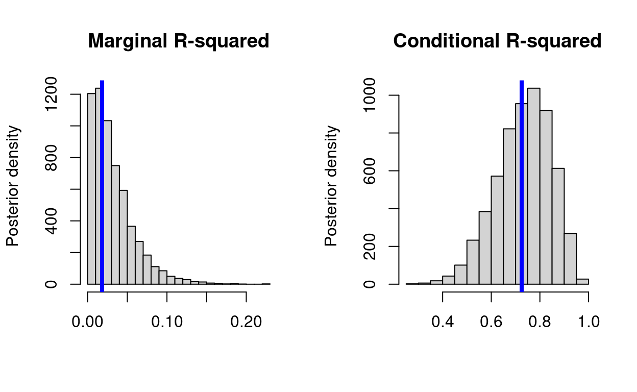
This plot shows the posterior \(R^2_{GLMM}\) distributions for both the marginal
and conditional cases, with the point estimates generated with glmer shown as
vertical blue lines. Personally, I find it to be a bit more informative and
intuitive to think of \(R^2\) as a probability distribution that integrates
uncertainty in its component parameters. That said, it is unconventional to
represent \(R^2\) in this way, which could compromise the ease with which this
handy statistic can be explained to the uninitiated (e.g. first year biology
undergraduates). But, being a derived parameter, those wishing to generate a
posterior can do so relatively easily.