Dealing with proportion data on the interval \([0, 1]\) is tricky. I realized this while trying to explain variation in vegetation cover. Unfortunately this is a true proportion, and can’t be made into a binary response. Further, true 0’s and 1’s rule out beta regression. You could arcsine square root transform the data (but shouldn’t; Warton and Hui 2011). Enter zero-and-one inflated beta regression.
The zero-and-one-inflated beta distribution facilitates modeling fractional or proportional data that contains both 0’s and 1’s (Ospina and Ferrari 2010 - highly recommended). The general idea is to model the response variable (call it \(y\)) as a mixture of Bernoulli and beta distributions, from which the true 0’s and 1’s, and the values between 0 and 1 are generated, respectively. The probability density function is
\[ f_{\text{ZOIB}}(y; \alpha, \gamma, \mu, \phi) = \left\{ \begin{array}{lr} \alpha(1 - \gamma) & y = 0\\ \alpha \gamma & y = 1\\ (1 - \alpha)f(y; \mu, \phi) & 0 < y < 1 \end{array} \right. \]
where \(0 < \alpha, \gamma, \mu < 1\), and \(\phi>0\). \(f(y; \mu, \phi)\) is the probability density function for the beta distribution, parameterized in terms of its mean \(\mu\) and precision \(\phi\):
\[f_{\text{beta}}(y; \mu, \phi) = \dfrac{\Gamma(\phi)}{\Gamma(\mu \phi) \Gamma((1 - \mu)\phi)} y^{\mu \phi - 1} (1 - y)^{(1 - \mu)\phi - 1}\]
\(\alpha\) is a mixture parameter that determines the extent to which the Bernoulli or beta component dominates the pdf. \(\gamma\) determines the probability that \(y=1\) if it comes from the Bernoulli component. \(\mu\) and \(\phi\) are the expected value and the precision for the beta component, which is usually parameterized in terms of \(p\) and \(q\) (Ferrari and Cribari-Neto 2004). \(\mu = \frac{p}{p + q}\), and \(\phi=p+q\).
Although ecologists often deal with proportion data, I haven’t found any examples of 0 & 1 inflated beta regression in the ecological literature. Closest thing I’ve found was Nishii and Tanaka (2012) who take a different approach, where values between 0 and 1 are modeled as logit-normal.
Here’s a quick demo in JAGS with simulated data. For simplicity, I’ll assume 1) there is one covariate that increases the expected value at the same rate for both the Bernoulli and beta components s.t. \(\mu = \gamma\), and 2) the Bernoulli component dominates extreme values of the covariate, where the expected value is near 0 or 1.
library(rjags)
library(ggmcmc)
library(reshape2)

set.seed(1234)
n <- 60
x <- runif(n, -3, 3)
a0 <- -3
a1 <- 0
a2 <- 1
antilogit <- function(x){
  exp(x) / (1 + exp(x))
}
alpha <- antilogit(a0 + a1 * x + a2 * x^2)

b0 <- 0
b1 <- 2
mu <- antilogit(b0 + b1 * x)
phi <- 5
p <- mu * phi
q <- phi - mu * phi

y.discrete <- rbinom(n, 1, alpha)
y <- rep(NA, n)
for (i in 1:n){
  if (y.discrete[i] == 1){
    y[i] <- rbinom(1, 1, mu[i])
  } else {
    y[i] <- rbeta(1, p[i], q[i])
  }
}

# split the data into discrete and continuous components
y.d <- ifelse(y == 1 | y == 0, y, NA)
y.discrete <- ifelse(is.na(y.d), 0, 1)
y.d <- y.d[!is.na(y.d)]
x.d <- x[y.discrete == 1]
n.discrete <- length(y.d)

which.cont <- which(y < 1 & y > 0)
y.c <- ifelse(y < 1 & y > 0, y, NA)
y.c <- y.c[!is.na(y.c)]
n.cont <- length(y.c)
x.c <- x[which.cont]
Now we can specify our model in JAGS, following the factorization of the likelihood given by Ospina and Ferrari (2010), estimate our parameters, and see how well the model performs.
# write model
cat(
  "
  model{
  # priors
  a0 ~ dnorm(0, .001)
  a1 ~ dnorm(0, .001)
  a2 ~ dnorm(0, .001)
  b0 ~ dnorm(0, .001)
  b1 ~ dnorm(0, .001)
  t0 ~ dnorm(0, .01)
  tau <- exp(t0)

  # likelihood for alpha
  for (i in 1:n){
    logit(alpha[i]) <- a0 + a1 * x[i] + a2 * x[i] ^ 2
    y.discrete[i] ~ dbern(alpha[i])
  }

  # likelihood for gamma
  for (i in 1:n.discrete){
    y.d[i] ~ dbern(mu[i])
    logit(mu[i]) <- b0 + b1 * x.d[i]
  }

  # likelihood for mu and tau
  for (i in 1:n.cont){
    y.c[i] ~ dbeta(p[i], q[i])
    p[i] <- mu2[i] * tau
    q[i] <- (1 - mu2[i]) * tau
    logit(mu2[i]) <- b0 + b1 * x.c[i]
  }
  }
  ", file="beinf.txt"
)

jd <- list(x=x, y.d=y.d, y.c=y.c, y.discrete = y.discrete,
           n.discrete=n.discrete, n.cont = n.cont,
           x.d = x.d, x.c=x.c, n=n)
mod <- jags.model("beinf.txt", data= jd, n.chains=3, n.adapt=1000)
Compiling model graph
Resolving undeclared variables
Allocating nodes
Graph information:
Observed stochastic nodes: 120
Unobserved stochastic nodes: 6
Total graph size: 849
Initializing model
|
| | 0%
|
|+ | 2%
|
|++ | 4%
|
|+++ | 6%
|
|++++ | 8%
|
|+++++ | 10%
|
|++++++ | 12%
|
|+++++++ | 14%
|
|++++++++ | 16%
|
|+++++++++ | 18%
|
|++++++++++ | 20%
|
|+++++++++++ | 22%
|
|++++++++++++ | 24%
|
|+++++++++++++ | 26%
|
|++++++++++++++ | 28%
|
|+++++++++++++++ | 30%
|
|++++++++++++++++ | 32%
|
|+++++++++++++++++ | 34%
|
|++++++++++++++++++ | 36%
|
|+++++++++++++++++++ | 38%
|
|++++++++++++++++++++ | 40%
|
|+++++++++++++++++++++ | 42%
|
|++++++++++++++++++++++ | 44%
|
|+++++++++++++++++++++++ | 46%
|
|++++++++++++++++++++++++ | 48%
|
|+++++++++++++++++++++++++ | 50%
|
|++++++++++++++++++++++++++ | 52%
|
|+++++++++++++++++++++++++++ | 54%
|
|++++++++++++++++++++++++++++ | 56%
|
|+++++++++++++++++++++++++++++ | 58%
|
|++++++++++++++++++++++++++++++ | 60%
|
|+++++++++++++++++++++++++++++++ | 62%
|
|++++++++++++++++++++++++++++++++ | 64%
|
|+++++++++++++++++++++++++++++++++ | 66%
|
|++++++++++++++++++++++++++++++++++ | 68%
|
|+++++++++++++++++++++++++++++++++++ | 70%
|
|++++++++++++++++++++++++++++++++++++ | 72%
|
|+++++++++++++++++++++++++++++++++++++ | 74%
|
|++++++++++++++++++++++++++++++++++++++ | 76%
|
|+++++++++++++++++++++++++++++++++++++++ | 78%
|
|++++++++++++++++++++++++++++++++++++++++ | 80%
|
|+++++++++++++++++++++++++++++++++++++++++ | 82%
|
|++++++++++++++++++++++++++++++++++++++++++ | 84%
|
|+++++++++++++++++++++++++++++++++++++++++++ | 86%
|
|++++++++++++++++++++++++++++++++++++++++++++ | 88%
|
|+++++++++++++++++++++++++++++++++++++++++++++ | 90%
|
|++++++++++++++++++++++++++++++++++++++++++++++ | 92%
|
|+++++++++++++++++++++++++++++++++++++++++++++++ | 94%
|
|++++++++++++++++++++++++++++++++++++++++++++++++ | 96%
|
|+++++++++++++++++++++++++++++++++++++++++++++++++ | 98%
|
|++++++++++++++++++++++++++++++++++++++++++++++++++| 100%out <- coda.samples(mod, c("a0", "a1", "a2", "b0", "b1", "tau"),
n.iter=6000)
  |
  |                                                  |   0%
  |
  |*                                                 |   2%
  |
  |**                                                |   4%
  |
  |***                                               |   6%
  |
  |****                                              |   8%
  |
  |*****                                             |  10%
  |
  |******                                            |  12%
  |
  |*******                                           |  14%
  |
  |********                                          |  16%
  |
  |*********                                         |  18%
  |
  |**********                                        |  20%
  |
  |***********                                       |  22%
  |
  |************                                      |  24%
  |
  |*************                                     |  26%
  |
  |**************                                    |  28%
  |
  |***************                                   |  30%
  |
  |****************                                  |  32%
  |
  |*****************                                 |  34%
  |
  |******************                                |  36%
  |
  |*******************                               |  38%
  |
  |********************                              |  40%
  |
  |*********************                             |  42%
  |
  |**********************                            |  44%
  |
  |***********************                           |  46%
  |
  |************************                          |  48%
  |
  |*************************                         |  50%
  |
  |**************************                        |  52%
  |
  |***************************                       |  54%
  |
  |****************************                      |  56%
  |
  |*****************************                     |  58%
  |
  |******************************                    |  60%
  |
  |*******************************                   |  62%
  |
  |********************************                  |  64%
  |
  |*********************************                 |  66%
  |
  |**********************************                |  68%
  |
  |***********************************               |  70%
  |
  |************************************              |  72%
  |
  |*************************************             |  74%
  |
  |**************************************            |  76%
  |
  |***************************************           |  78%
  |
  |****************************************          |  80%
  |
  |*****************************************         |  82%
  |
  |******************************************        |  84%
  |
  |*******************************************       |  86%
  |
  |********************************************      |  88%
  |
  |*********************************************     |  90%
  |
  |**********************************************    |  92%
  |
  |***********************************************   |  94%
  |
  |************************************************  |  96%
  |
  |************************************************* |  98%
  |
  |**************************************************| 100%
ggd <- ggs(out)
a0.post <- subset(ggd, Parameter == "a0")$value
a1.post <- subset(ggd, Parameter == "a1")$value
a2.post <- subset(ggd, Parameter == "a2")$value
n.stored <- length(a2.post)
P.discrete <- array(dim=c(n.stored, n))
for (i in 1:n){
P.discrete[, i] <- antilogit(a0.post + a1.post * x[i] + a2.post * x[i] ^ 2)
}
pdd <- melt(P.discrete, varnames = c("iteration", "site"),
value.name = "Pr.discrete")
pdd$x <- x[pdd$site]
b0.post <- subset(ggd, Parameter == "b0")$value
b1.post <- subset(ggd, Parameter == "b1")$value
expect <- array(dim=c(n.stored, n))
for (i in 1:n){
expect[, i] <- antilogit(b0.post + b1.post * x[i])
}
exd <- melt(expect, varnames=c("iteration", "site"), value.name = "Expectation")
exd$x <- x[exd$site]
obsd <- data.frame(x=x, y=y,
component = factor(ifelse(y < 1 & y > 0,
"Continuous", "Discrete")))
trued <- data.frame(x=x, mu=mu)
ggplot(pdd) +
geom_line(aes(x=x, y=Pr.discrete, group=iteration),
alpha=0.05, color="grey") +
geom_line(aes(x=x, y=Expectation, group=iteration),
data=exd, color="blue", alpha=0.05) +
geom_point(aes(x=x, y=y, fill=component),
data=obsd, size=3, color="black",
position = position_jitter(width=0, height=.01), pch=21) +
scale_fill_manual(values = c("red", "white"), "Component") +
ylab("y") +
geom_line(aes(x=x, y=mu),
data=trued, color="green", linetype="dashed") +
theme_bw()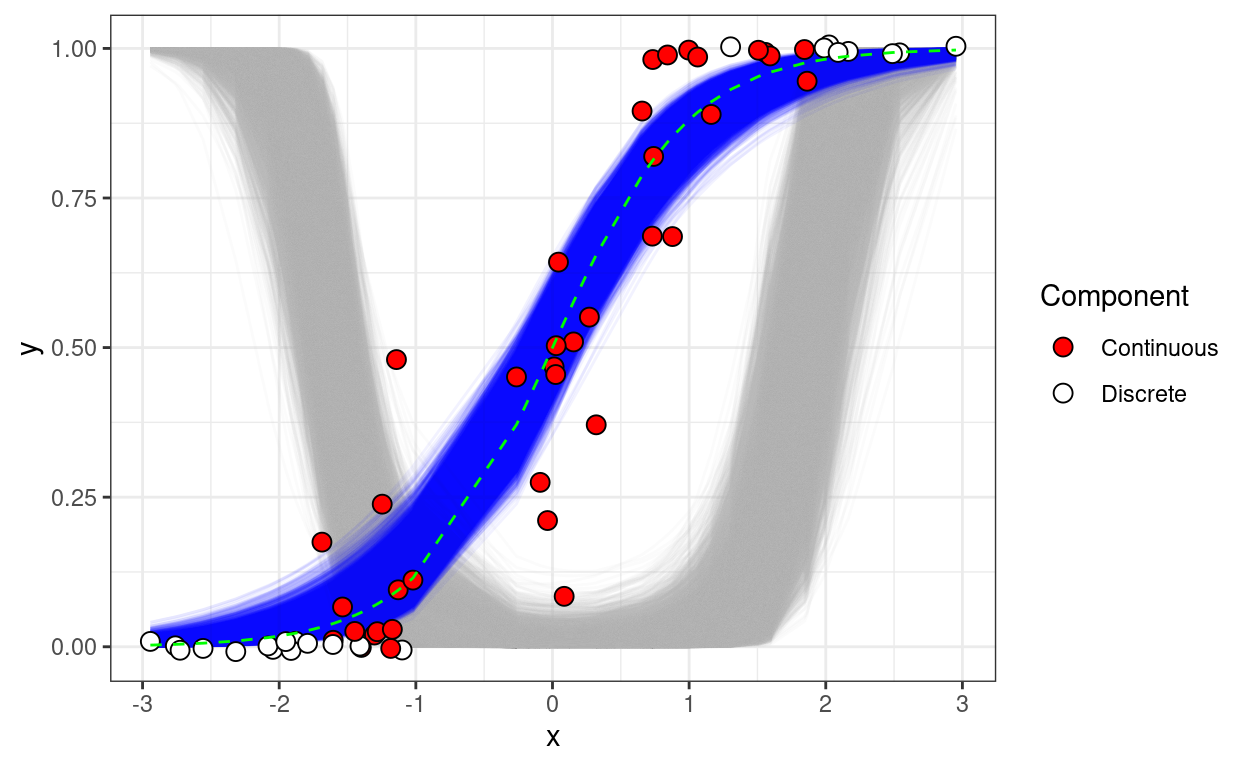
Here the posterior probability that \(y\) comes from the discrete Bernoulli component is shown in grey, and the posterior expected value for both the Bernoulli and beta components across values of the covariate are shown in blue. The dashed green line shows the true expected value that was used to generate the data. Finally, the observed data are shown as jittered points, color coded as being derived from the continuous beta component, or the discrete Bernoulli component.