Here, I’ll describe a Bayesian approach for estimation and correction for covariate measurement error using a latent-variable based errors-in-variables model, that one might use when there is uncertainty in the covariate for a linear model. Recall that this matters because error in covariate measurements tends to bias slope estimates towards zero.
For what follows, we’ll assume a simple linear regression, in which continuous covariates are measured with error. True covariate values are considered latent variables, with repeated measurements of covariate values arising from a normal distribution with a mean equal to the true value, and some measurement error \(\sigma_x\), such that \(\epsilon_x \sim \text{Normal}(0, \sigma_x)\) and \(\epsilon_y \sim \text{Normal}(0, \sigma_y)\), where \(\epsilon_x\) represents error in the covariate, and \(\epsilon_y\) represents error in the response variable.
We assume that for sample unit \(i\) and repeat measurement \(j\):
\[ x^{obs}_{ij} \sim \text{Normal}(x_i, \sigma_x) \]
\[ y_i \sim \text{Normal}(\alpha + \beta x_i, \sigma_y) \]
The trick here is to use repeated measurements of the covariates to estimate and correct for measurement error. In order for this to be valid, the true covariate values cannot vary across repeat measurements. If the covariate was individual weight, you would have to ensure that the true weight did not vary across repeat measurements (for me, frogs urinating during handling would violate this assumption).
Below, I’ll simulate some data of this type in R. I’m assuming that we randomly
select some sampling units to remeasure covariate values, and each is
remeasured n.reps times.
library(rstan)
rstan_options(auto_write = TRUE)
options(mc.cores = parallel::detectCores())

set.seed(1234)
n.reps <- 3
n.repeated <- 10
n <- 30

# true covariate values
x <- runif(n, -3, 3)
y <- x + rnorm(n)  # alpha=0, beta=1, sdy=1

# random subset to perform repeat covariate measurements
which.repeated <- sample(n, n.repeated)
xsd <- .5  # measurement error
xerr <- rnorm(n + (n.repeated * (n.reps - 1)), 0, xsd)

# indx assigns measurements to sample units
indx <- c(1:n, rep(which.repeated, each = n.reps - 1))
indx <- sort(indx)
nobs <- length(indx)
xobs <- x[indx] + xerr
plot(x[indx], xobs,
    xlab = "True covariate value",
    ylab = "Observed covariate value")
abline(0, 1, lty = 2)
segments(x0 = x[indx], x1 = x[indx],
    y0 = x[indx], y1 = xobs, col = "red")
abline(v = x[which.repeated], col = "green", lty = 3)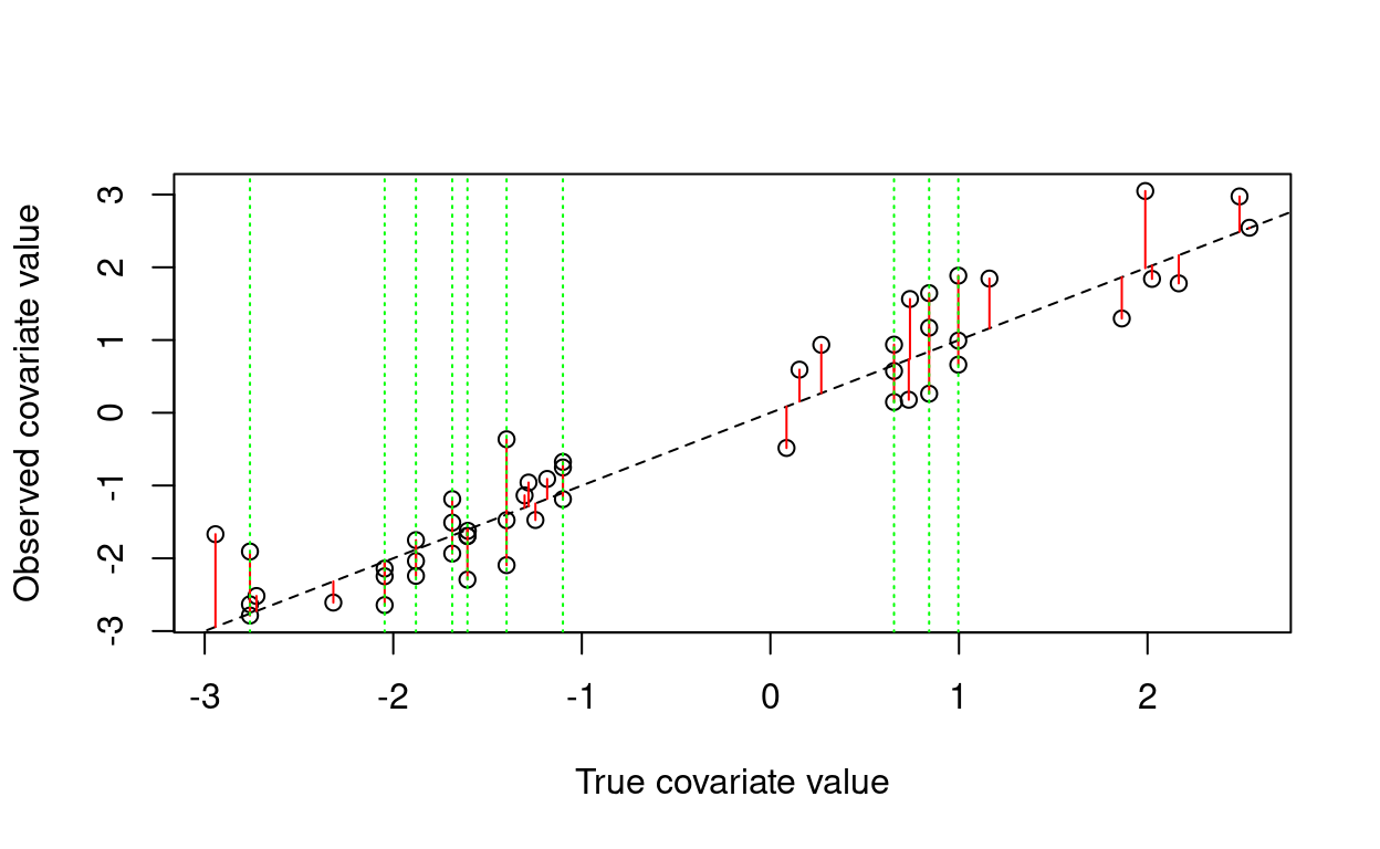
Here, the discrepancy due to measurement error is shown as a red segment, and the sample units that were measured three times are highlighted with green dashed lines.
I’ll use stan to estimate the model parameters, because I’ll be refitting the model to new data sets repeatedly below, and Stan is faster than JAGS for these models.
# write the .stan file
cat("
data{
  int n;
  int nobs;
  real xobs[nobs];
  real y[n];
  int indx[nobs];
}

parameters {
  real alpha;
  real beta;
  real<lower=0> sigmay;
  real<lower=0> sigmax;
  real x[n];
}

model {
  // priors
  alpha ~ normal(0, 1);
  beta ~ normal(0, 1);
  sigmay ~ normal(0, 1);
  sigmax ~ normal(0, 1);

  // model structure
  for (i in 1:nobs){
    xobs[i] ~ normal(x[indx[i]], sigmax);
  }
  for (i in 1:n){
    y[i] ~ normal(alpha + beta*x[i], sigmay);
  }
}

  ",
    file = "latent_x.stan")
With the model specified, estimate the parameters.
How did we do? Let’s compare the true vs. estimated covariate values for each sample unit.
posteriors <- rstan::extract(mod1)

# highest density interval helper function (thanks to Joe Mihaljevic)
HDI <- function(values, percent = 0.95) {
    sorted <- sort(values)
    index <- floor(percent * length(sorted))
    nCI <- length(sorted) - index
    width <- rep(0, nCI)
    for (i in 1:nCI) {
        width[i] <- sorted[i + index] - sorted[i]
    }
    HDImin <- sorted[which.min(width)]
    HDImax <- sorted[which.min(width) + index]
    HDIlim <- c(HDImin, HDImax)
    return(HDIlim)
}

# comparing estimated true x values to actual x values
Xd <- array(dim = c(n, 3))
for (i in 1:n) {
    Xd[i, 1:2] <- HDI(posteriors$x[, i])
    Xd[i, 3] <- median(posteriors$x[, i])
}

lims <- c(min(Xd), max(Xd))
plot(x, Xd[, 3], xlab = "True covariate value",
    ylab = "Estimated covariate value",
    col = "purple", pch = 19, ylim = lims)
abline(0, 1, lty = 2)
segments(x0 = x, x1 = x, y0 = Xd[, 1], y1 = Xd[, 2], col = "purple")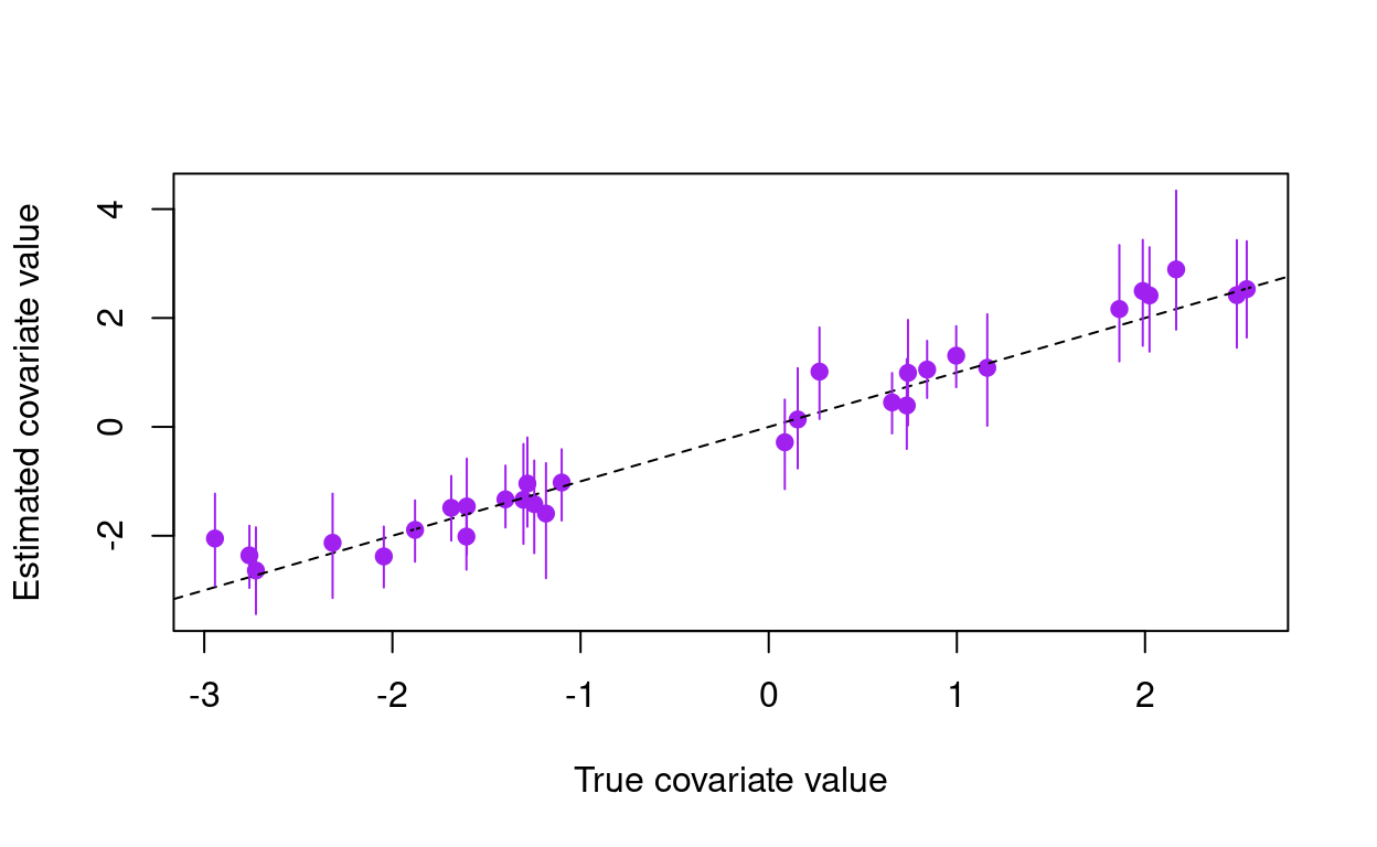
Here purple marks the posterior for the covariate values, and the dashed black line shows the one-to-one line that we would expect if the estimates exactly matched the true values. In addition to estimating the true covariate values, we may wish to check to see how well we estimated the standard deviation of the measurement error in our covariate.
hist(posteriors$sigmax, breaks = 30,
    main = "Posterior for measurement error",
    xlab = "Measurement standard deviation")
abline(v = xsd, col = "red", lwd = 2)
legend("topright", legend = "True value", col = "red",
    lty = 1, bty = "n", lwd = 2)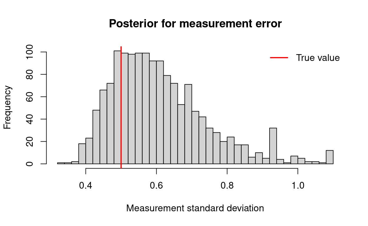
How many sample units need repeat measurements?
You may want to know how many sample units need to be repeatedly measured to adequately estimate the degree of covariate measurement error. For instance, if \(\sigma_x = 1\), how does the precision in our estimate of \(\sigma_x\) improve as more sample units are repeatedly measured? Let’s see what happens when we repeatedly measure covariate values for \(1, 2, ..., N\) randomly selected sampling units.
n.repeated <- 1:n

# store the HDI and mode for the estimate of sigmax in an array
post.sdx <- array(dim = c(length(n.repeated), 3))
for (i in n.repeated) {
    n.repeats <- i
    which.repeated <- sample(n, n.repeats)
    xerr <- rnorm(n + (n.repeats * (n.reps - 1)), 0, xsd)
    indx <- c(1:n, rep(which.repeated, each = n.reps - 1))
    indx <- sort(indx)
    nobs <- length(indx)
    xobs <- x[indx] + xerr
    stan_d <- c("y", "xobs", "nobs", "n", "indx")
    mod <- stan(fit = mod1, data = stan_d, chains = chains,
        iter = iter, thin = thin)
    posteriors <- extract(mod)
    post.sdx[i, 1:2] <- HDI(posteriors$sigmax)
    post.sdx[i, 3] <- median(posteriors$sigmax)
}
# Plot the relationship b/t number of sampling units revisited & sdx
plot(x = n.repeated, y = rep(xsd, length(n.repeated)),
type = "l", lty = 2,
ylim = c(0, max(post.sdx)),
xlab = "Number of sampling units measured three times",
ylab = "Estimated measurement error")
segments(x0 = n.repeated, x1 = n.repeated,
y0 = post.sdx[, 1], y1 = post.sdx[, 2],
col = "red")
points(x = n.repeated, y = post.sdx[, 3], col = "red")
legend("topright", legend = c("True value", "Posterior estimate"),
col = c("black", "red"), lty = c(2, 1),
pch = c(NA, 1), bty = "n")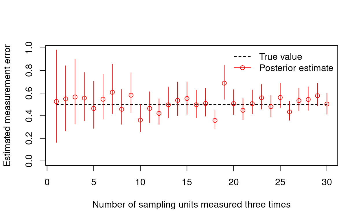
Looking at this plot, you could eyeball the number of sample units that should be remeasured when designing a study. Realistically, you might want to explore how this number depends on the true amount of measurement error, and also simulate multiple realizations (rather than just one) for each scenario. Using a similar approach, you might also evaluate whether it’s more efficient to remeasure more sample units, or invest in more repeated measurements per sample unit.