Maxwell B. Joseph: Categorical spatial data extraction around buffered points in R

Quantifying categorical spatial data (e.g. land cover) around points can be done in a variety of ways, some of which require considerable amounts of patience, clicking around, and/or cash for a license. Here’s a bit of code that I cobbled together to quickly extract land cover data from the National Land Cover Database for a buffered point between Denver and Boulder - two cities in the state of Colorado.

First, get data using the FedData package:

library(knitr)
library(raster)
library(FedData)
library(rgdal)

site_df <- data.frame(city = c('Denver', 'Boulder'), 
                      lat = c(39.7392, 40.0150), 
                      lon = c(-104.9903, -105.2705))
midpoint <- data.frame(lat = mean(site_df$lat), 
                       lon = mean(site_df$lon))

# create spatial point data frame
coordinates(site_df) <- ~lon + lat
proj4string(site_df) <- CRS("+proj=longlat +ellps=WGS84 +datum=WGS84")

coordinates(midpoint) <- ~lon + lat
proj4string(midpoint) <- CRS("+proj=longlat +ellps=WGS84 +datum=WGS84")

nlcd_raster <- get_nlcd(site_df, 
                        label = 'categorial-extraction', 
                        year = 2011, 
                        extraction.dir = '.')

# reproject midpoint to raster's crs
midpoint <- spTransform(midpoint, projection(nlcd_raster))

buffer_distance_meters <- 5000

# visualize buffered point and land cover data
buff_shp <- buffer(midpoint, buffer_distance_meters)
plot(buff_shp) # I will plot over this, but it sets the plotting extent
plot(nlcd_raster, add = TRUE)
plot(buff_shp, add = TRUE)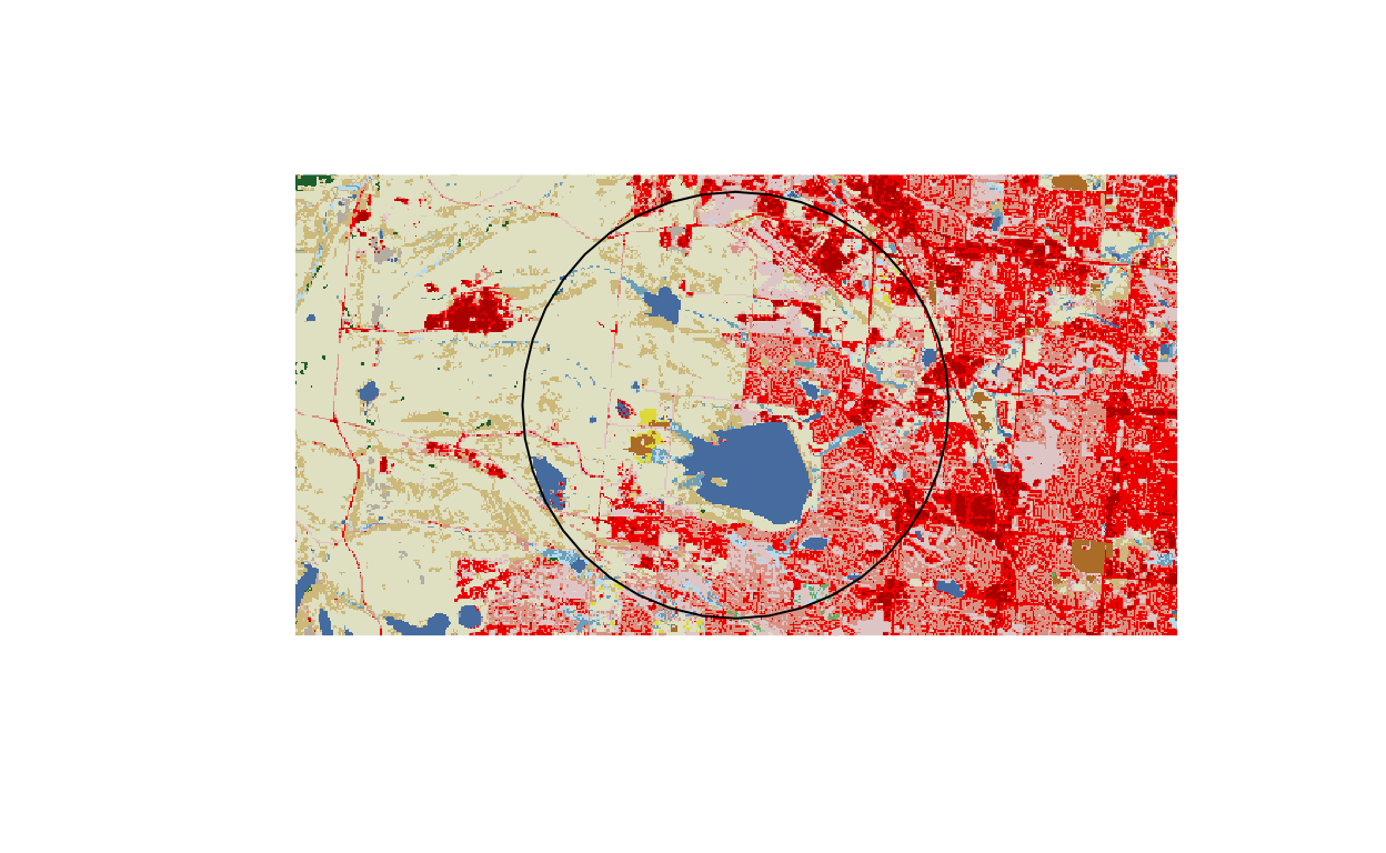

Now, we can use raster::extract to extract raster data around our point within some buffer, specified in meters.

landcover <- extract(nlcd_raster, midpoint, buffer = buffer_distance_meters)

But this object does not immediately provide the proportions of each cover type. Instead, it contains values from the cells within the buffer:

str(landcover)

List of 1
 $ : num [1:87274] 22 21 21 21 22 22 21 21 21 21 ...

We can get the proportions of each class within the buffer as follows:

landcover_proportions <- lapply(landcover, function(x) {
  counts_x <- table(x)
  proportions_x <- prop.table(counts_x)
  sort(proportions_x)
  })
sort(unlist(landcover_proportions))

          43           42           41           31           82 
8.020716e-05 1.604143e-04 1.294773e-03 2.406215e-03 3.781195e-03 
          81           90           95           24           52 
5.202007e-03 1.184774e-02 1.911222e-02 3.251828e-02 6.305429e-02 
          11           21           23           22           71 
8.288837e-02 1.150056e-01 1.328804e-01 1.734766e-01 3.562917e-01

Resources

Categorical spatial data extraction around buffered points in R

Corrections

Reuse