Gaussian process (GP) models are computationally demanding for large datasets. Much work has been done to avoid expensive matrix operations that arise in parameter estimation with larger datasets via sparse and/or reduced rank covariance matrices (Datta et al. 2016 provide a nice review). What follows is an implementation of a spatial Gaussian predictive process Poisson GLM in Stan, following Finley et al. 2009: Improving the performance of predictive process modeling for large datasets, with a comparison to a full rank GP model in terms of execution time and MCMC efficiency.
Generative model
Assume we have \(n\) spatially referenced counts \(y(s)\) made at spatial locations \(s_1, s_2, ..., s_n\), which depend on a latent mean zero Gaussian process with an isotropic stationary exponential covariance function:
\[y(s) \sim \text{Poisson}(\text{exp}(X^T(s) \beta + w(s)))\]
\[w(s) \sim GP(0, C(d))\]
\[[C(d)]_{i, j} = \eta^2 \text{exp}(- d_{ij} \phi)) + I(i = j) \sigma^2\]
where \(y(s)\) is the response at location \(s\), \(X\) is an \(n \times p\) design matrix, \(\beta\) is a length \(p\) parameter vector, \(\sigma^2\) is a “nugget” parameter, \(\eta^2\) is the variance parameter of the Gaussian process, \(d_{ij}\) is a spatial distance between locations \(s_i\) and \(s_j\), and \(\phi\) determines how quickly the correlation in \(w\) decays as distance increases. For simplicity, the point locations are uniformly distributed in a 2d unit square spatial region.
To estimate this model in a Bayesian context, we might be faced with taking a Cholesky decomposition of the \(n \times n\) matrix \(C(d)\) at every iteration in an MCMC algorithm, a costly operation for large \(n\).
Gaussian predictive process representation
Computational benefits of Gaussian predictive process models arise from the estimation of the latent Gaussian process at \(m << n\) locations (knots). Instead of taking the Cholesky factorization of the \(n \times n\) covariance matrix, we instead factorize the \(m \times m\) covariance matrix corresponding to the covariance in the latent spatial process among knots. Knot placement is a non-trivial topic, but for the purpose of illustration let’s place knots on a grid over the spatial region of interest. Note that here the knots are fixed, but it is possible to model knot locations stochastically as in Guhaniyogi et al. 2012.
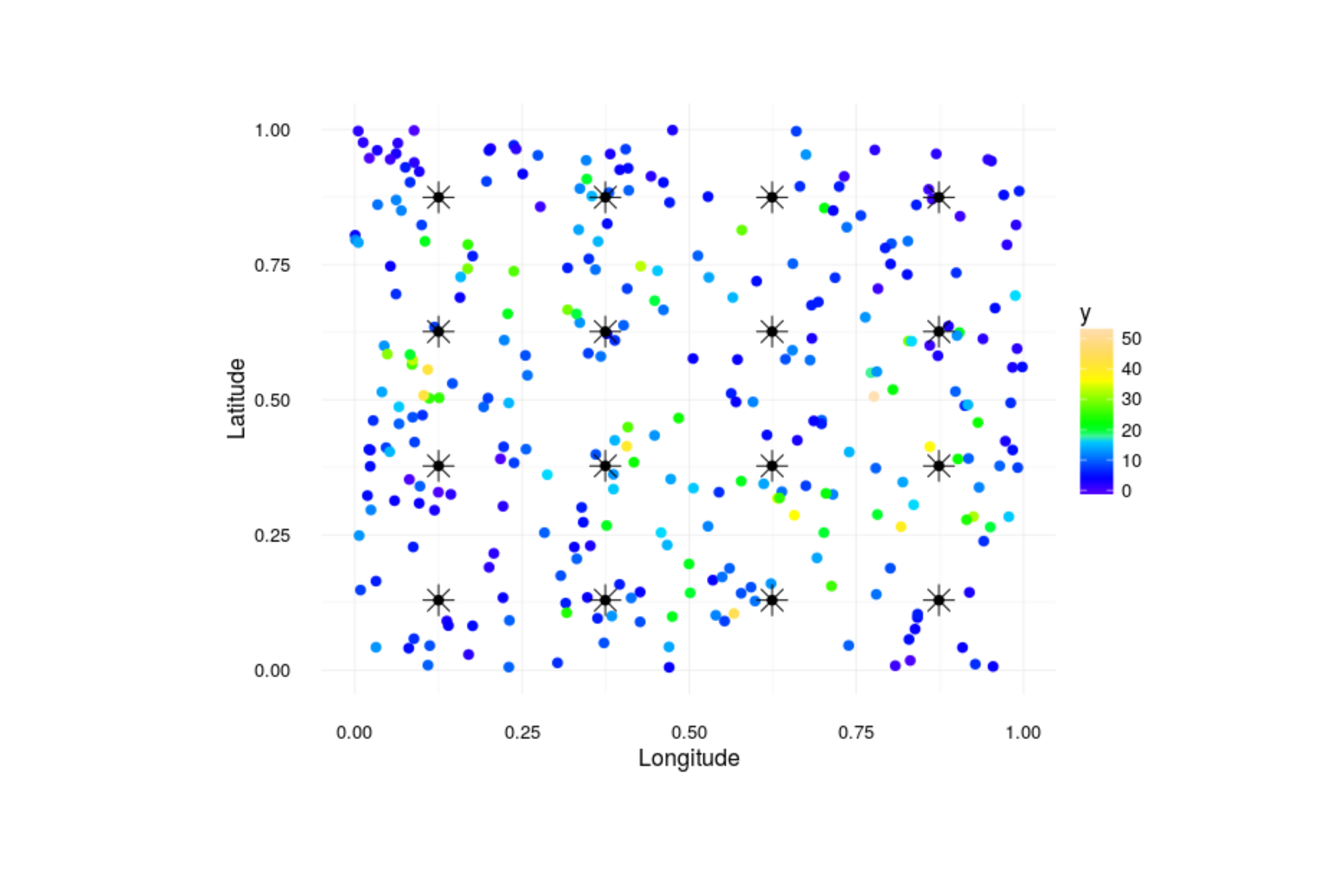
Knots are shown as stars and the points are observations.
We will replace \(w\) above with an estimate of \(w\) that is derived from a reduced rank representation of the latent spatial process. Below, the vector \(\tilde{\boldsymbol{\epsilon}}\) corrects for bias (underestimation of \(\eta\) and overestimation of \(\sigma\)) as an extension of Banerjee et al. 2008, and \(\mathcal{C}^T(\theta) \mathcal{C}^{*-1}(\theta)\) relates \(w\) at desired point locations to the value of the latent GP at the knot locations, where \(\mathcal{C}^T(\theta)\) is an \(n \times m\) matrix that gets multiplied by the inverse of the \(m \times m\) covariance matrix for the latent spatial process at the knots. For a complete and general description see Finley et al. 2009, but here is the jist of the univariate model:
\[\boldsymbol{Y} \sim \text{Poisson}(\boldsymbol{X} \beta + \mathcal{C}^T(\theta) \mathcal{C}^{*-1}(\theta)\boldsymbol{w^*} + \tilde{\boldsymbol{\epsilon}})\]
\[\boldsymbol{w^*} \sim GP(0, \mathcal{C}^*(\theta))\]
\[\tilde{\epsilon}(s) \stackrel{indep}{\sim} N(0, C(s, s) - \mathcal{c}^T(\theta) \mathcal{C}^{*-1}(\theta))\mathcal{c}(\theta)\]
with priors for \(\eta\), \(\sigma\), and \(\phi\) completing a Bayesian specification.
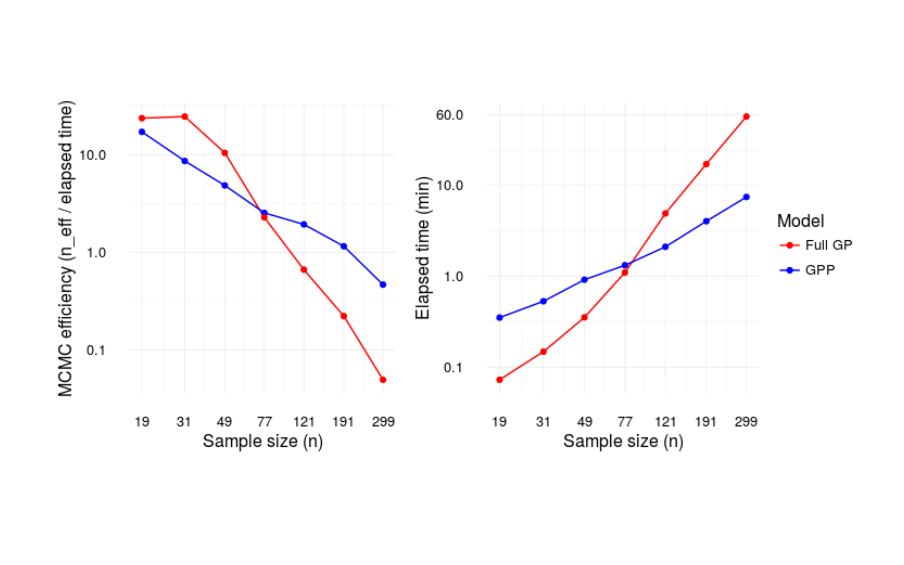
This approach scales well for larger datasets relative to a full rank GP model. Comparing the number of effective samples per unit time for the two approaches across a range of sample sizes, the GPP executes more quickly and is more efficient for larger datasets. Code for this simulation is available on GitHub: https://github.com/mbjoseph/gpp-speed-test.
Relevant papers