Multilevel modeling of community composition with imperfect detection

A guest post by Joe Mihaljevic.

This is a guest post generously provided by Joe Mihaljevic.

A common goal of community ecology is to understand how and why species composition shifts across space. Common techniques to determine which environmental covariates might lead to such shifts typically rely on ordination of community data to reduce the amount of data. These techniques include redundancy analysis (RDA), canonical correspondence analysis (CCA), and nonmetric multi-dimensional scaling (NMDS), each paired with permutation tests. However, these ordination techniques do not discern species-level covariate effects, making it difficult to attribute community-level pattern shifts to species-level changes (Jackson et al. 2012). Jackson et al. (2012) propose a hierarchical modeling framework as an alternative, which we extend in this post to correct for imperfect detection.

Multilevel models can estimate species-level random and fixed covariate effects to determine the relative contribution of environmental covariates to changing composition across space (Jackson et al. 2012). For presence/absence data, such models are often formulated as:

\[y_{q} \sim \text{Bernoulli}(\psi_{q})\]

\[\psi_{q} = logit^{-1}(\alpha_{spp[q]} + b_{spp[q]} x_{site[q]})\]

\[\alpha_{spp[q]} \sim N(\mu_{\alpha}, \sigma_{intercept}^2)\]

\[b_{spp[q]} \sim N(\mu_{b}, \sigma_{slope}^2)\]

Here \(y_q\) is a vector of presences/absence of each species at each site (\(q=1, ... , nm,\) where \(n\) is the number of species and \(m\) the number of sites). This model can be extended to incorporate multiple covariates.

We are interested in whether species respond differently to environmental gradients (e.g. elevation, temperature, precipitation). If this is the case, then we expect community composition changes along such gradients. Concretely, we are interested in whether \(\sigma_{slope}^2\) for any covariate differs from zero.

Jackson et al. (2012) provide code for a maximum likelihood implementation of their model with data from Southern Appalachian understory herbs using the R package lme4. Here we present a simple extension of Jackson and colleague’s work, correcting for detection error with repeat surveys (i.e. multi-species occupancy modeling). Specifically, the above model could be changed slightly to:

\[y_{q} \sim \text{Binomial}(z_q p_{spp[q]}, j_q)\]

\[z_q \sim \text{Bernoulli}(\psi_q)\]

\[\psi_{q} = logit^{-1}(\alpha_{spp[q]} + b_{spp[q]} x_{site[q]})\]

\[\alpha_{spp[q]} \sim N(\mu_{\alpha}, \sigma_{intercept}^2)\]

\[b_{spp[q]} \sim N(\mu_{b}, \sigma_{slope}^2)\]

Now \(y_q\) is the number of times each species is observed at each site over \(j\) surveys. \(p_{spp[q]}\) represents the species-specific probability of detection when the species is present, and \(z_q\) represents the ‘true’ occurence of the species, a Bernoulli random variable with probability, \(\psi_q\).

To demonstrate the method, we simulate data for a 20 species community across 100 sites with 4 repeat surveys. We assume that three site-level environmental covariates were measured, two of which have variable affects on occurrence probabilities (i.e. random effects), and one of which has consistent effects for all species (i.e. a fixed effect). We also assumed that species-specific detection probabilities varied, but were independent of environmental covariates.

library(reshape2)
library(ggplot2)

################################################
# Simulate data
################################################

Nsite <- 100
Ncov <- 3
Nspecies <- 20
J <- 4
set.seed(1234)

# species-specific intercepts:
alpha <- rnorm(Nspecies, 0, 1)

# covariate values
Xcov <- matrix(rnorm(Nsite*Ncov, 0, 2),
               nrow=Nsite, ncol=Ncov)

# I'll assume 2 of the 3 covariates have effects that vary among species
Beta <- array(c(rnorm(Nspecies, 0, 2),
                rnorm(Nspecies, -1, 1),
                rep(1, Nspecies)
                ),
              dim=c(Nspecies, Ncov)
              )

# species-specific detection probs
p0 <- plogis(rnorm(Nspecies, 1, 0.5))

#### Occupancy states ####
Yobs <- array(0, dim = c(Nspecies, Nsite)) # Simulated observations

for(n in 1:Nspecies){
  for(k in 1:Nsite){
    lpsi <- alpha[n] + Beta[n, ] %*% Xcov[k, ] # Covariate effects on occurrence
    psi <- 1/(1+exp(-lpsi)) #anti-logit

    z <- rbinom(1, 1, psi) # True Occupancy
    Yobs[n, k] <- rbinom(1, J, p0[n] * z) # Observed Occupancy
  }
}

################################################
# Format data for model
################################################
# X needs to have repeated covariates for each species, long form
X <- array(0, dim=c(Nsite*Nspecies, Ncov))
t <- 1; i <- 1
TT <- Nsite
while(i <= Nspecies){
  X[t:TT, ] <- Xcov
  t <- t+Nsite
  TT <- TT + Nsite
  i <- i+1
}

# Species
Species <- rep(c(1:Nspecies), each=Nsite)

# Observations/data:
Y <- NULL
for(i in 1:Nspecies){
  Y <- c(Y, Yobs[i, ])
}

# All sites surveyed same # times:
J <- rep(J, times=Nspecies*Nsite)

# Number of total observations
Nobs <- Nspecies*Nsite

Each species has a coefficient for each covariate that describes how the probability of occurrence responds. In one case, all species have the same response:

beta_df <- melt(Beta, varnames = c('Species', 'Covariate'))
ggplot(beta_df) + 
  geom_point(aes(value, Species)) + 
  facet_wrap(~Covariate, nrow = 1) + 
  xlab('Coefficient value') + 
  ggtitle('Species-level coefficients for each covariate (facets)') + 
  theme_minimal()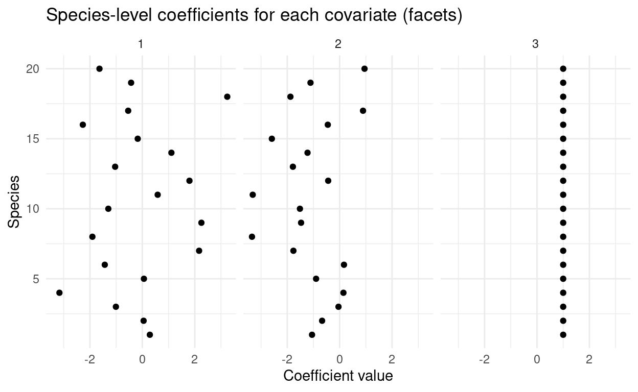

We fit the following model with JAGS with vague priors.

model {
  # Priors
  psi.mean ~ dbeta(1,1)
  p.detect.mean ~ dbeta(1,1)

  sd.psi ~ dunif(0,10)
  psi.tau <- pow(sd.psi, -2)

  sd.p.detect ~ dunif(0,10)
  p.detect.tau <- pow(sd.p.detect, -2)

  for(i in 1:Nspecies){
    alpha[i] ~ dnorm(logit(psi.mean), psi.tau)T(-12,12)
    lp.detect[i] ~ dnorm(logit(p.detect.mean), p.detect.tau)T(-12,12)
    p.detect[i] <- exp(lp.detect[i]) / (1 + exp(lp.detect[i]))
  }

  for(j in 1:Ncov){
    mean.beta[j] ~ dnorm(0, 0.01)
    sd.beta[j] ~ dunif(0, 10)
    tau.beta[j] <- pow(sd.beta[j]+0.001, -2)
    for(i in 1:Nspecies){
      betas[i,j] ~ dnorm(mean.beta[j], tau.beta[j])
    }
  }

  # Likelihood
  for(i in 1:Nobs){
    logit(psi[i]) <- alpha[Species[i]] + inprod(betas[Species[i],], X[i, ])
    z[i] ~ dbern(psi[i])
    Y[i] ~ dbinom(z[i] * p.detect[Species[i]], J[i])
  }
}

Using information theory, specifically Watanabe-Akaike information criteria (WAIC), we compared this model, which assumes all covariates have random effects, to all combination of models varying whether each covariate has fixed or random effects. See this GitHub repository for all model statements and code.

A model that assumes all covariates have random effects, and the data-generating model, in which only covariates 1 and 2 have random effects, performed the best, but were indistinguishable from one another:

This result makes sense because the model with all random effects is able to recover species-specific responses to site-level covariates very well:

However, this model estimates that the 95% HDI of \(\sigma_{slope}\) of covariate 3 includes zero, indicating that this covariate effectively has a fixed, rather than random effect among species.

Thus, we could conclude that the first two covariates have random effects, while the third covariate has a fixed effect. This means that composition shifts along gradients of covariates 1 and 2. We can visualize the relative contribution of covariate 1 and 2’s random effects to composition using ordination, as discussed in Jackson et al. (2012). To do this, we compare the linear predictor (i.e. \(\text{logit}^{-1}(\psi_q)\)) of the best model that includes only significant random effects to a model that does not have any random effects.

The code to extract linear predictors and ordinate the community is provided on GitHub.