Behind the paper: Neural hierarchical models of ecological populations

A high-level overview, an example, and a call to action.

This post gives some background and a demo for the paper “Neural hierarchical models of ecological populations” out today in Ecology Letters (Joseph 2020).

Deep learning and model-based ecological inference may seem like totally separate pursuits. Yet, if you think about deep learning as a set of tools to approximate functions, it’s not much of a leap to begin seeing opportunities to unite deep learning with some standard ecological modeling approaches.

Hierarchical models

Hierarchical models have been around for a while, and are now one of the workhorse methods of modern quantitative ecology (e.g., occupancy models, capture-recapture models, N-mixture models, animal movement models, state-space models, etc.). Hierarchical models combine:

1. A data model \([y \mid z, \theta]\) where we observe \(y\), that depends on a process \(z\), and parameter(s) \(\theta\),
2. A process model \([z \mid \theta]\), and
3. A parameter model \([\theta]\).

A posterior distribution of the unknowns, conditioned on the data is:

\[[z, \theta \mid y] = \dfrac{[y \mid z, \theta] \times [z \mid \theta] \times [\theta]}{[y]}.\]

We might also have some explanatory variables \(x\) that might tell us something about \(z\), \(\theta\), and/or \(y\).

Neural networks

Neural networks approximate functions. Off the shelf neural networks usually just map \(x\) to \(y\), and allow us to predict new values of \(y\) for new values of \(x\). Sometimes, predicting \(y\) is not really what we care about - we really want to learn something about a process \(z\) or some parameters \(\theta\).

Neural hierarchical models

We can parameterize a hierarchical model with a neural network to learn about \(z\). So, for example, if \(\theta\) represents the parameters of a neural network, then we can construct a process model \([z \mid \theta]\) where our input \(x\) is mapped to a process \(z\) by way of some neural network:

\[[z \mid \theta] = f(x, \theta),\]

where \(f\) is a neural network that maps \(x\) and \(\theta\) to some probabilistic model for \(z\) (here because \(x\) is observed, I’m not going to condition \(z\) on it on the left hand side of the equation - \(x\) is assumed to be constant and known without error).

Graphically, you might consider a state-space model where some inputs \(x\) are mapped to a state transition matrix (for an example with an animal movement model, see Appendix S2 in the paper):

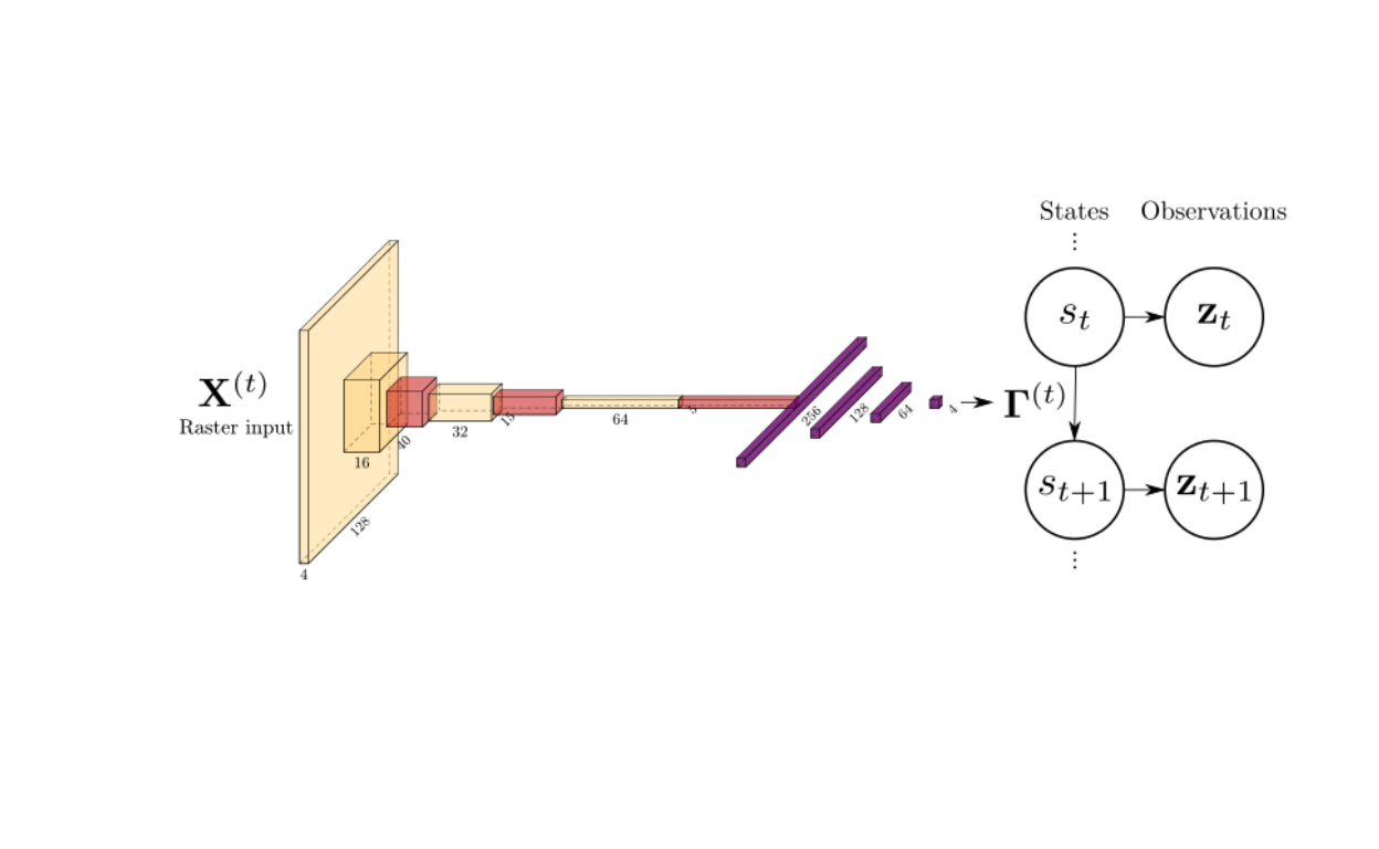
Figure 1: Using a convolutional neural network to map some input raster to a state transition matrix in a hidden Markov model

An example: a neural N-mixture model

An N-mixture model can be used to estimate latent integer-valued abundance when unmarked populations are repeatedly surveyed and it is assumed that detection of individuals is imperfect (Royle 2004). Assume that \(J\) spatial locations are each surveyed \(K\) times, in a short time interval for which it is reasonable to assume that the number of individuals is constant within locations \(j=1, ..., J\). Each spatial location has some continuous covariate value represented by \(x_j\), that relates to detection probabilities and expected abundance.

Observation model

Observations at site \(j\) in survey \(k\) yield counts of the number of unique individuals detected, denoted \(y_{j, k}\) for all \(j\) and all \(k\). Assuming that the detection of each individual is conditionally independent, and that each individual is detected with site-specific probability \(p_j\), the observations can be modeled with a Binomial distribution where the number of trials is the true (latent) population abundance \(n_j\):

\[y_{j, k} \sim \text{Binomial}(p_j, n_j).\]

Process model

The true population abundance \(n_j\) is treated as a Poisson random variable with expected value \(\lambda_j\):

\[n_j \sim \text{Poisson}(\lambda_j).\]

Parameter model

Heterogeneity among sites was accounted for using a single layer neural network that ingests the one dimensional covariate \(x_i\) for site \(i\), passes it through a single hidden layer, and outputs a two dimensional vector containing a detection probability \(p_i\) and the expected abundance \(\lambda_i\):

\[ \begin{bmatrix} \lambda_i \\ p_i \end{bmatrix} = f(x_i), \]

where \(f\) is a neural network with two dimensional output activations \(\vec{h}(x_i)\) computed via:

\[\vec{h}(x_i) = \vec{W}^{(2)} g(\vec{W}^{(1)} x_i ),\] and final outputs computed using the log and logit link functions for expected abundance and detection probability:

\[f(x_i) = \begin{bmatrix} \text{exp}(h_1(x_i)) \\ \text{logit}^{-1}(h_2(x_i)) \end{bmatrix}.\]

Here too \(\vec{W}^{(1)}\) is a parameter matrix that generates activations from the inputs, \(g\) is an activation function, and \(\vec{W}^{(2)}\) is a parameter matrix that maps the hidden layer to the outputs. Additionally \(h_1(x_i)\) is the first element of the output activation vector, and \(h_2(x_i)\) the second element.

Loss function

The negative log likelihood was used as the loss function, enumerating over a large range of potential values of the true abundance (from \(\min(y_j.)\) to \(5 \times \max(y_j.)\), where \(y_{j.}\) is a vector of counts of length \(K\)) to approximate the underlying infinite mixture model implied by the Poisson model of abundance (Royle 2004).

Simulating some data

First, load some python dependencies.

import matplotlib.pyplot as plt
import multiprocessing
import numpy as np
import torch
from torch import nn
from torch.distributions import Binomial, Poisson
from torch.utils.data import DataLoader, TensorDataset

Simulate data at nsite sites, with nrep repeat surveys. Here it’s assumed that there is one continuous site-level covariate \(x\) that has some nonlinear relationship with the expected number of individuals at a site.

np.random.seed(123456)
nsite = 200
nrep = 5
x = np.linspace(-2.5, 2.5, nsite, dtype=np.float32).reshape(-1,1)

# Draw f(x) from a Gaussian process
def kernel(x, theta):
    m, n = np.meshgrid(x, x)
    sqdist = abs(m-n)**2
    return np.exp(- theta * sqdist)

K = kernel(x, theta=.2)
L = np.linalg.cholesky(K + 1e-5* np.eye(nsite))
f_prior = np.dot(L, np.random.normal(size=(nsite, 1)))

Generate some abundance values from a Poisson distribution:

offset = 3
lam = np.exp(f_prior + offset)
n = np.random.poisson(lam)

plt.scatter(x, n, c='k', alpha=.3)
plt.plot(x, lam)
plt.xlabel('Covariate value')
plt.ylabel('True (latent) abundance')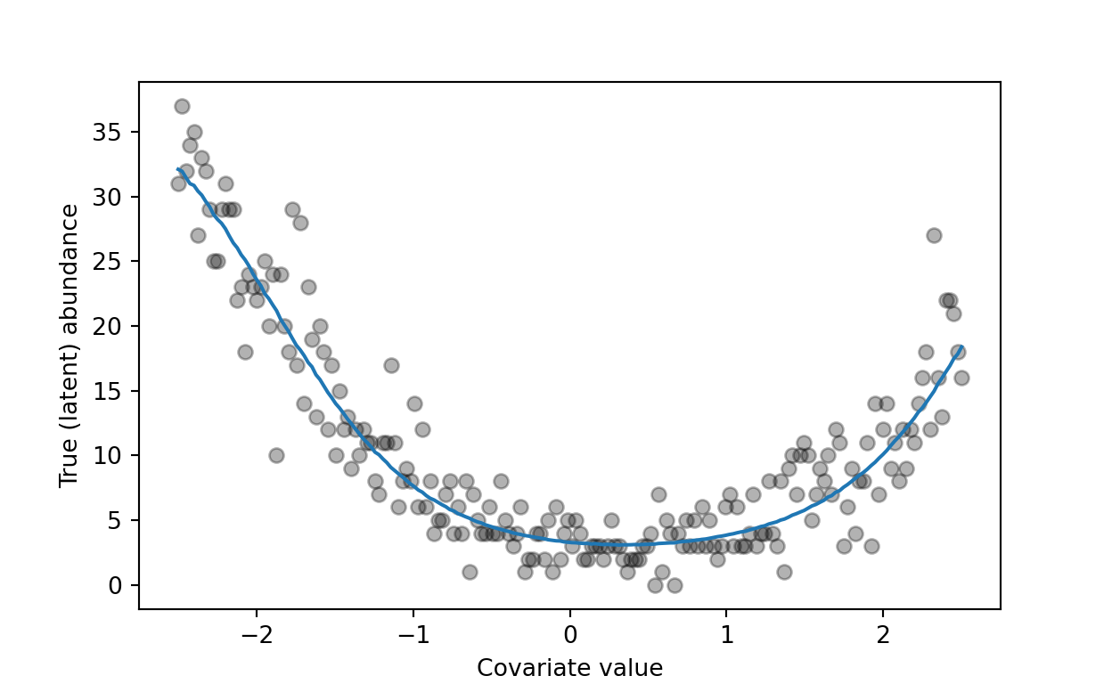

Figure 2: True relationship between latent abundance and the covariate, with sampled points.

For simplicity, assume that the probability of detection is constant across all sites and independent of \(x\).

pr_detection = np.array([0.5])
y = np.random.binomial(n=n, 
                       p=pr_detection, 
                       size=(nsite, nrep))

plt.plot(x, lam)
for i in range(nrep):
    plt.scatter(x, y[:, i], c='b', s=4, alpha=.3)    
plt.xlabel('Covariate value')
plt.ylabel('Observed counts')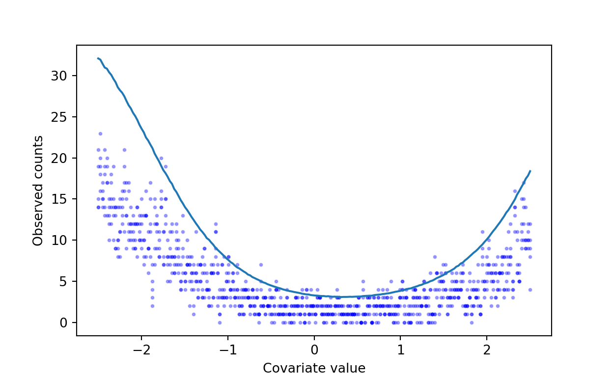

(#fig:gen_data)Observed counts as a function of the covariate value.

Defining a neural network

We will define a torch.nn.Module class for our neural network. This ingests \(x\) and outputs a value for \(\lambda\) and \(p\):

class Net(nn.Module):
    """ Neural N-mixture model 
    
    This is a neural network that ingests x and outputs:
    - lam(bda): expected abundance
    - p: detection probability
    """
    def __init__(self, hidden_size):
        super().__init__()
        self.fc1 = nn.Linear(1, hidden_size)
        self.fc2 = nn.Linear(hidden_size, 2)

    def forward(self, x):
        hidden_layer = torch.sigmoid(self.fc1(x))
        output = self.fc2(hidden_layer)
        lam = torch.exp(output[:, [0]])
        p = torch.sigmoid(output[:, [1]])
        return lam, p

Defining a loss function

We will use the negative log likelihood as our loss function:

def nmix_loss(y_obs, lambda_hat, p_hat, n_max):
    """ N-mixture loss.
    
    Args:
      y_obs (tensor): nsite by nrep count observation matrix
      lambda_hat (tensor): poisson abundance expected value
      p_hat (tensor): individual detection probability
      n_max (int): maximum abundance to consider
    
    Returns:
      negative log-likelihood (tensor)
    """
    batch_size, n_rep = y_obs.shape
    
    possible_n_vals = torch.arange(n_max).unsqueeze(0)
    n_logprob = Poisson(lambda_hat).log_prob(possible_n_vals)
    assert n_logprob.shape == (batch_size, n_max)
    
    y_dist = Binomial(
      possible_n_vals.view(1, 1, -1), 
      probs=p_hat.view(-1, 1, 1), 
      validate_args=False
    )
    y_obs = y_obs.unsqueeze(-1).repeat(1, 1, n_max)
    y_logprob = y_dist.log_prob(y_obs).sum(dim=1) # sum over repeat surveys
    assert y_logprob.shape == (batch_size, n_max)
    
    log_lik = torch.logsumexp(n_logprob + y_logprob, -1)
    return -log_lik

Preparing to train

Instantiate a model.

net = Net(hidden_size=32)
net

Create a data loader.

dataset = TensorDataset(torch.tensor(x).float(), torch.tensor(y))
dataloader = DataLoader(dataset, 
                        batch_size=16,
                        shuffle=True, 
                        num_workers=multiprocessing.cpu_count())

Instantiate an optimizer and choose the number of training epochs:

n_epoch = 1000
optimizer = torch.optim.Adam(net.parameters(), lr=0.01, weight_decay=1e-6)
running_loss = []

Training the model

Finally, train the model, visualizing the estimated relationship between \(x\) and \(N\) after every gradient update.

_ = plt.scatter(x, n, c='k')
_ = plt.xlabel('Covariate value')
_ = plt.ylabel('Abundance')
colors = plt.cm.viridis(np.linspace(0,1,n_epoch))
for i in range(n_epoch):
    for i_batch, xy in enumerate(dataloader):
        x_i, y_i = xy
        optimizer.zero_grad()
        lambda_i, p_i = net(x_i)
        nll = nmix_loss(y_i, lambda_i, p_i, n_max = 200)
        loss = torch.mean(nll)        
        loss.backward()
        optimizer.step()    # Does the update
        running_loss.append(loss.data.detach().numpy())
    lam_hat, p_hat = net(torch.from_numpy(x))
    lam_hat = lam_hat.detach().numpy()
    _ = plt.plot(x, lam_hat, color=colors[i], alpha=.1)
plt.show()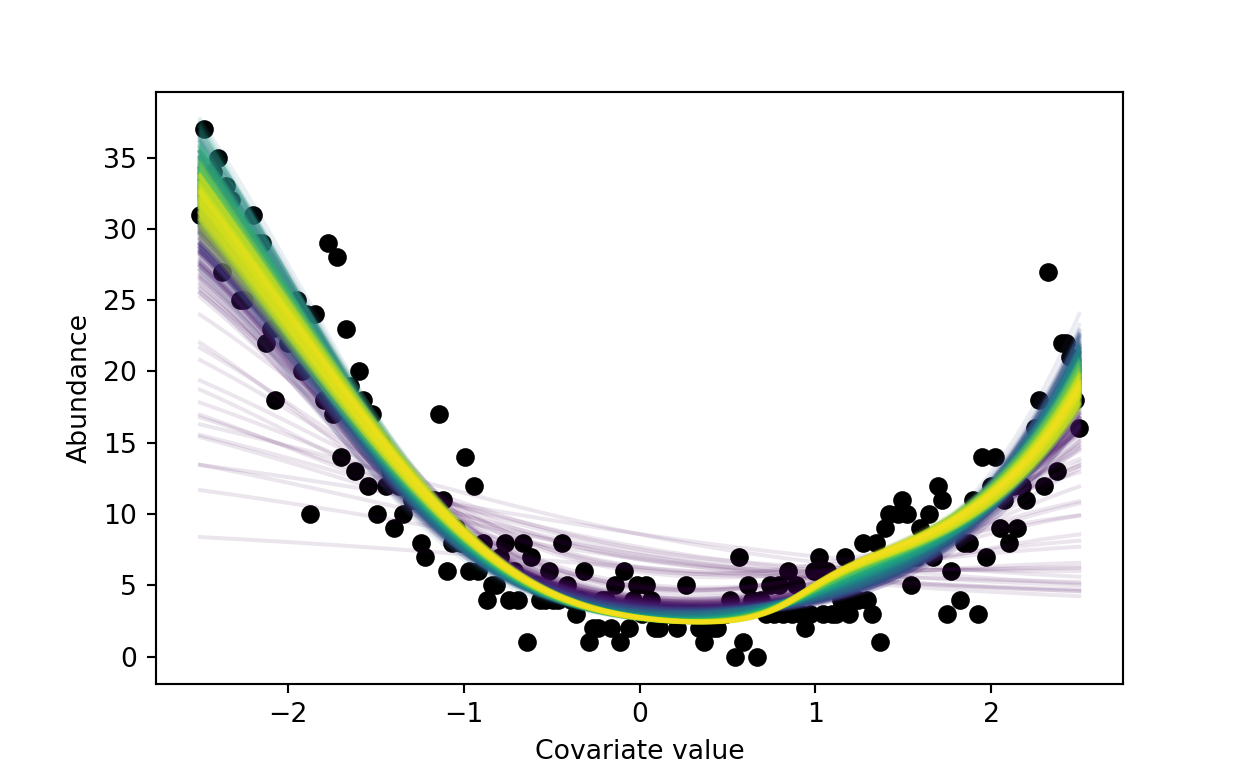

Figure 3: Estimated relationships between x and abundance as training progresses. Dark blue lines represent predictions from early training iterations, and green/yellow represent middle/late training iterations.

Figure 3: Estimated relationships between x and abundance as training progresses. Dark blue lines represent predictions from early training iterations, and green/yellow represent middle/late training iterations.

Visualize loss:

n_step = len(running_loss)
_ = plt.scatter(x=np.arange(n_step), y=running_loss, s=2,
                color=plt.cm.viridis(np.linspace(0,1,n_step)))
_ = plt.xlabel('Number of training iterations')
_ = plt.ylabel('N-mixture loss')
plt.show()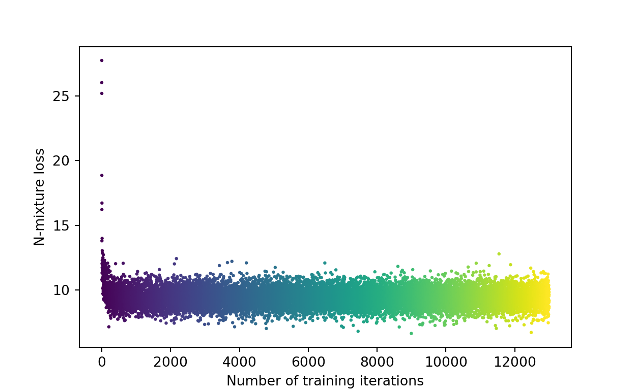

Figure 4: Training loss over time. Each point corresponds to the loss after a gradient update.

Figure 4: Training loss over time. Each point corresponds to the loss after a gradient update.

More on implementing hierarchical models

If you are interested in digging into the details of how to build these models, check out the companion repository on GitHub, which has all of the code required to reproduce the paper, as well as links to Jupyter Notebooks (thanks Binder!) to play with some toy occupancy, capture-recapture, and N-mixture models: https://github.com/mbjoseph/neuralecology

Parting thoughts

Deep learning is somewhat of a mystery to many ecologists. Those who are currently applying it have done some amazing things (like counting plants and animals in imagery). But, I worry that as a community, ecologists are thinking about deep learning too narrowly.

We can look to hydrology and physics to get a sense for how we can advance science with deep learning. Here are a few key papers that are shaping my thinking around this topic, which might help motivate future work in science-based deep learning for ecology:

• Karpatne, Anuj, et al. “Physics-guided neural networks (pgnn): An application in lake temperature modeling.” arXiv preprint arXiv:1710.11431 (2017). link
• Raissi, Maziar. “Deep hidden physics models: Deep learning of nonlinear partial differential equations.” The Journal of Machine Learning Research 19.1 (2018): 932-955. link
• Rangapuram, Syama Sundar, et al. “Deep state space models for time series forecasting.” Advances in neural information processing systems. 2018. link
• Rackauckas, Christopher, et al. “Universal Differential Equations for Scientific Machine Learning.” arXiv preprint arXiv:2001.04385 (2020). link