Discrete parameters can be a major stumbling block for ecologists using Stan, because you need to marginalize over the latent discrete parameters (e.g., “alive/dead”, “occupied/not occupied”, “infected/not infected”, etc.). This post demonstrates how to do it, step by step for a simple example. I’ll try to make it clear what we are doing along the way, as we work towards a model that we can represent in Stan.
Consider a Bayesian site occupancy model. We want to estimate occurrence states (presence or absence) using observed detection/non-detection data (MacKenzie et al. 2002). For sites \(i=1, ...,N\) we have \(K\) replicate sampling occasions. On each sampling occasion, we visit site \(i\) and look for a critter (a bug, a bird, a plant, etc.).
Represent the number of sampling occasions where we detected the critter at site \(i\) as \(y_i\). So if we see the critter on two surveys, \(y_i = 2\).
We assume that if a site is occupied (\(z_i=1\)), we detect the animal with probability \(p\). If a site is not occupied (\(z_i=0\)), we can’t observe it.
How a BUGS/JAGS/NIMBLE user might write the model
We can write the observation model for site \(i\) as:
\[y_i \sim \text{Binomial}(K, p z_i).\]
And our prior for the occupancy state of site \(i\) is:
\[z_i \sim \text{Bernoulli}(\psi),\]
where \(\psi\) is the probability of occupancy.
A Bayesian model specification is completed by assigning priors to the remaining parameters:
\[p \sim \text{Uniform}(0, 1),\] \[\psi \sim \text{Uniform}(0, 1).\]
Square bracket probability notation
Let’s rewrite the model in a different way. First, I want to introduce a different notation for our observation model:
\[[y_i \mid p, z_i] = \text{Binomial}(y_i \mid K, p z_i).\]
In this notation, square brackets represent probability mass or density functions (for discrete or continuous quantities, respectively). Here, \([y_i \mid p, z_i]\) is the probability mass function of \(y_i\) conditioned on the parameters \(p\) and \(z_i\).
If we assume that the observations \(y_{1:N} = y_1, ..., y_N\) for each site are conditionally independent, we can write the observation model for all sites \(1:N\) as:
\[[y_{1:N} \mid p, z_{1:N}] = \prod_{i=1}^N [y_i \mid p, z_i],\]
which follows from the definition of the joint distribution of independent random variables.
We can rewrite the rest of the model in the same notation. The state model for site \(i\) becomes:
\[[z_i \mid \psi] = \text{Bernoulli}(z_i \mid \psi).\]
And, again if we assume that the occupancy states for site \(i=1, ..., N\) are conditionally independent, then we can write down the state model for all sites as:
\[[z_{1:N} \mid \psi] = \prod_{i=1}^N \text{Bernoulli}(z_i \mid \psi).\]
Finally, we can write the priors in square bracket notation:
\[[\psi] = \text{Uniform}(\psi \mid 0, 1),\]
\[[p] = \text{Uniform}(p \mid 0, 1).\]
Writing the joint distribution
We are working towards a model specification that we can use in Stan, which means we need the log of the joint distribution of data and parameters.
The “joint distribution of data and parameters” is the numerator in Bayes’ theorem, which gives us an expression for the posterior probability distribution of parameters \(\theta\) given data \(y\):
\[[\theta \mid y] = \dfrac{[y, \theta]}{[y]}.\]
In this example, our parameters \(\theta\) are:
- \(z_{1:N}\): the occupancy states
- \(p\): the detection probability
- \(\psi\): the occupancy probability
The data consist of the counts \(y_{1:N}\).
So our joint distribution is:
\[[y_{1:N}, \theta] = [y_{1:N}, z_{1:N}, p, \psi],\]
We can factor this using the rules of conditional probability and the components we worked out in the previous section. First, recognize that:
- \(y\) depends on \(p\) and \(z\),
- \(z\) depends on \(\psi\), and
- \(p\) and \(\psi\) don’t depend on any other parameters:
\[[y_{1:N}, z_{1:N}, p, \psi] = [y_{1:N} \mid p, z_{1:N}] \times [z_{1:N} \mid \psi] \times [p, \psi].\]
Then, recall that we can represent the joint probability distribution for the capture histories and states as a product of site-specific terms:
\[[y_{1:N}, z_{1:N}, p, \psi] = \prod_{i=1}^N [y_i \mid p, z_i] \times \prod_{i=1}^N [z_i \mid \psi] \times [p, \psi].\]
We can simplify this a little:
\[[y_{1:N}, z_{1:N}, p, \psi] = \prod_{i=1}^N [y_i \mid p, z_i] [z_i \mid \psi] \times [p, \psi].\]
Last, we have independent priors for \(p\) and \(\psi\), so we can write the joint distribution as:
\[[y_{1:N}, z_{1:N}, p, \psi] = \prod_{i=1}^N [y_i \mid p, z_i] [z_i \mid \psi] \times [p] [\psi].\]
In case that is confusing, it can also be useful to visualize this same dependence structure graphically.
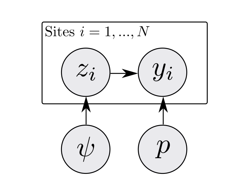
Figure 1: A directed acyclic graph for an occupancy model. Arrows represent dependence (e.g., p -> y means y depends on p).
This is almost in a form that we can use in Stan. But we need to get rid of \(z\) from the model. It’s a discrete parameter, and Stan needs continuous parameters.
Marginalizing over discrete parameters
To get rid of our discrete parameter \(z\), we need to marginalize it out of the model. In general, if you have a joint distribution for \(y\) and \(z\) that depends on \(\theta\), you obtain the marginal distribution of \(y\) by summing the joint distribution over all possible values of \(z\):
\[[y \mid \theta] = \sum_{z} [y, z \mid \theta].\]
In our case, for the \(i^{th}\) site, this means that we need to marginalize over \(z_i\) as follows:
\[[y_i \mid p, \psi] = \sum_{z_i=0}^1 [y_i, z_i \mid p, \psi].\]
We are summing over all possible values of \(z_i\). In this case there are two (\(z_i\) can be 0 or 1).
We can factor the joint distribution:
\[[y_i \mid p, \psi] = \sum_{z_i=0}^1 [y_i \mid p, z_i] [z_i \mid \psi].\]
This is:
\[[y_i \mid p, \psi] = [y_i \mid p, z_i=0] [z_i=0 \mid \psi] + [y_i \mid p, z_i=1] [z_i=1 \mid \psi].\]
Earlier we said \(\psi\) is the probability that \(z_i = 1\). So, \(1-\psi\) is the probability that \(z_i=0\):
\[[y_i \mid p, \psi] = (1 - \psi) [y_i \mid p, z_i=0] + \psi [y_i \mid p, z_i=1].\]
We can also simplify the observation model for unoccupied sites. Because we assume that there are no false positive detections, unoccupied sites (\(z_i=0\)) can only generate zero counts for \(y_i\) (or, you could say that \(y_i\) is identically zero if \(z_i=0\)). We can then write this as:
\[[y_i \mid p, \psi] = (1 - \psi) I(y_i=0) + \psi [y_i \mid p, z_i=1],\]
where \(I(y_i=0)\) is an indicator function that is equal to one if \(y_i=0\), and otherwise is equal to zero.
It might be more intuitive to write this as:
\[[y_i \mid p, \psi] = \begin{cases} \psi [y_i \mid p, z_i=1], & \text{for } y_i > 0\\ \psi [y_i \mid p, z_i=1] + 1 - \psi, & \text{for } y_i = 0 \end{cases}\]
We can make this even more explicit by bringing back in the fact that our probability model for \(y_i\) is Binomial:
\[[y_i \mid p, \psi] = \begin{cases} \psi \text{Binomial}(y_i \mid p), & \text{for } y_i > 0\\ \psi \text{Binomial}(y_i \mid p) + 1 - \psi, & \text{for } y_i = 0 \end{cases}\]
Great - we just marginalized \(z_i\) out of the model.
Let’s circle back to the joint distribution and see what it looks like now. Previously we had:
\[[y_{1:N}, z_{1:N}, p, \psi] = \prod_{i=1}^N [y_i \mid p, z_i] [z_i \mid \psi] \times [p] [\psi].\]
Now, if we marginalize over \(z\) for every site, we’d be computing:
\[[y_{1:N}, p, \psi] = \prod_{i=1}^N \Big( \sum_{z_i=0}^1 [y_i \mid p, z_i] [z_i \mid \psi] \Big) \times [p] [\psi],\] \[ = \prod_{i=1}^N [y_i \mid p, \psi] \times [p] [\psi].\]
This joint distribution is something we can work with in Stan. The last thing we need to do is write down the log of the joint distribution, and translate that into Stan’s syntax.
The log of the joint distribution
We are going to specify the joint distribution in Stan on the log scale. Take the log of our joint distribution:
\[\log([y_{1:N}, p, \psi]) = \log \Bigg(\prod_{i=1}^N [y_i \mid p, \psi] \times [p] [\psi] \Bigg),\]
and by “\(\log\)” I mean the natural log.
Recall that the log of a product is the sum of logs: \(\log(ab) = \log(a) + \log(b)\)). We can apply this rule and find that:
\[\log([y_{1:N}, p, \psi]) = \sum_{i=1}^N \log [y_i \mid p, \psi] + \log[p] + \log[\psi].\]
Let’s think about how to represent \(\log [y_i \mid p, \psi]\). Recall from before that:
\[[y_i \mid p, \psi] = \begin{cases} \psi \text{Binomial}(y_i \mid p), & \text{for } y_i > 0\\ \psi \text{Binomial}(y_i \mid p) + 1 - \psi, & \text{for } y_i = 0 \end{cases}\]
Taking logarithms, we get:
\[\log [y_i \mid p, \psi] = \begin{cases} \log \big( \psi \text{Binomial}(y_i \mid p) \big), & \text{for } y_i > 0\\ \log \big( \psi \text{Binomial}(y_i \mid p) + 1 - \psi \big), & \text{for } y_i = 0 \end{cases}\]
Recalling rules about logs of products, we can rewrite this as:
\[\log [y_i \mid p, \psi] = \begin{cases} \log \psi + \log(\text{Binomial}(y_i \mid p)), & \text{for } y_i > 0\\ \log \big( \psi \text{Binomial}(y_i \mid p) + 1 - \psi \big), & \text{for } y_i = 0 \end{cases}\]
Stan has a function called binomial_lpmf (“binomial log probability mass function”) that gives us exactly what we need to compute \(\log(\text{Binomial}(y_i \mid p))\) above.
To make this connection clear, let’s rewrite this as:
\[\log [y_i \mid p, \psi] = \begin{cases} \log \psi + \text{binomial_lpmf}(y_i \mid p), & \text{for } y_i > 0\\ \log \big( \psi \text{Binomial}(y_i \mid p) + 1 - \psi \big), & \text{for } y_i = 0 \end{cases}\]
Then, let’s re-write the case where \(y_i=0\) as:
\[\log [y_i \mid p, \psi] = \begin{cases} \log \psi + \text{binomial_lpmf}(y_i \mid p), & \text{for } y_i > 0\\ \log \big( e^{\log(\psi \text{Binomial}(y_i \mid p))} + e^{\log(1 - \psi)} \big), & \text{for } y_i = 0 \end{cases}\]
This is true because \(e^{\log(x)}=x\).
Then, apply the rule about \(\log(ab) = \log a + \log b\) again:
\[\log [y_i \mid p, \psi] = \begin{cases} \log \psi + \text{binomial_lpmf}(y_i \mid p), & \text{for } y_i > 0\\ \log \big( e^{\log \psi + \text{binomial_lpmf}(y_i \mid p)} + e^{\log(1 - \psi)} \big), & \text{for } y_i = 0 \end{cases} \]
At this point, we are going to bring in the LogSumExp trick, which gives us a computationally stable way to compute terms like \(\log(\sum_i \exp(x_i))\).
Stan has a function called log_sum_exp that does this for us, and it takes the terms to sum on the log scale as inputs.
Let’s rewrite the model for the data with this function:
\[\log [y_i \mid p, \psi] = \begin{cases} \log \psi + \text{binomial_lpmf}(y_i \mid p), & y_i > 0\\ \text{log_sum_exp}(\log \psi + \text{binomial_lpmf}(y_i \mid p),\; \log(1 - \psi)), & y_i = 0 \end{cases} \]
Translating our model to Stan
Here’s the Stan model (written for clarity, not computational efficiency):
data {
  int<lower = 1> N;
  int<lower = 1> K;
  int<lower = 0, upper = K> y[N];
}

parameters {
  real<lower = 0, upper = 1> p;
  real<lower = 0, upper = 1> psi;
}

transformed parameters {
  vector[N] log_lik;

  for (i in 1:N) {
    if (y[i] > 0) {
      log_lik[i] = log(psi) + binomial_lpmf(y[i] | K, p);
    } else {
      log_lik[i] = log_sum_exp(
        log(psi) + binomial_lpmf(y[i] | K, p),
        log1m(psi)
      );
    }
  }
}

model {
  target += sum(log_lik);
  target += uniform_lpdf(p | 0, 1);
  target += uniform_lpdf(psi | 0, 1);
}
The observation model
We symbolically represented the observation model as:
\[\log [y_i \mid p, \psi] = \begin{cases} \log \psi + \text{binomial_lpmf}(y_i \mid p), & y_i > 0\\ \text{log_sum_exp}(\log \psi + \text{binomial_lpmf}(y_i \mid p),\; \log(1 - \psi)), & y_i = 0 \end{cases}\]
In Stan syntax, we are storing \(\log [y_i \mid p, \psi]\) in the \(i^{th}\) element of the vector log_lik.
We used an if-statement to deal with the different cases:
...
    if (y[i] > 0) {
      log_lik[i] = log(psi) + binomial_lpmf(y[i] | K, p);
    } else {
      log_lik[i] = log_sum_exp(
        log(psi) + binomial_lpmf(y[i] | K, p),
        log1m(psi)
      );
    }
...
The log joint distribution and target +=
Notice how in the model block, we used target += syntax to add things to the log joint distribution:
...
model {
  target += sum(log_lik);
  target += uniform_lpdf(p | 0, 1);
  target += uniform_lpdf(psi | 0, 1);
}
...
These terms correspond to the log joint distribution that we represented symbolically as
\[\log([y_{1:N}, p, \psi]) = \sum_{i=1}^N \log [y_i \mid p, \psi] + \log[p] + \log[\psi].\]
Bringing it all together
To recap, to go from our model specification with discrete parameters to a model that we can use in Stan, we did the following:
- Wrote the joint distribution of our model
- Marginalized discrete parameter(s) out of the joint distribution
- Took the log of the joint distribution
- Translated the log of the joint distribution into Stan code
This general approach applies to a variety of models, but occupancy models provide a simple example.
More resources
- The Stan documentation has some great content on marginalization of discrete parameters: https://mc-stan.org/docs/2_18/stan-users-guide/latent-discrete-parameterization.html
- Bob Carpenter put together a great case study for multi-species occupancy models in Stan, which provides a step up in complexity from this single-species model: https://mc-stan.org/users/documentation/case-studies/dorazio-royle-occupancy.html
- There are a ton of ecological models with discrete parameters that Hiroki Itô has translated to Stan from the book “Bayesian Population Analysis using WinBUGS — A Hierarchical Perspective” (2012) by Marc Kéry and Michael Schaub (Kéry and Schaub 2011): https://github.com/stan-dev/example-models/tree/master/BPA
- Most of the example spatial capture-recapture models from the 2013 book Spatial Capture-Recapture by Royle, Chandler, Gardner, and Sollmann (Royle et al. 2013) have also been translated to Stan: https://github.com/mbjoseph/scr-stan
- This post demonstrated how to marginalize symbolically (or “on paper” I guess), but there is another great blog post by Jacob Socolar that focuses on JAGS to Stan code translation (and includes a marginal model implementation in JAGS): https://github.com/jsocolar/occupancyModels